


Where do the peaks in the impedance of a flange come from?
When you are computing wakepotentials and impedances of a beampipe flange,
you will see not decaying signals in the wakepotentials and therefore peaks in the
impedance.
This writeup is an attempt to explain what kind of fields are responsible for these.
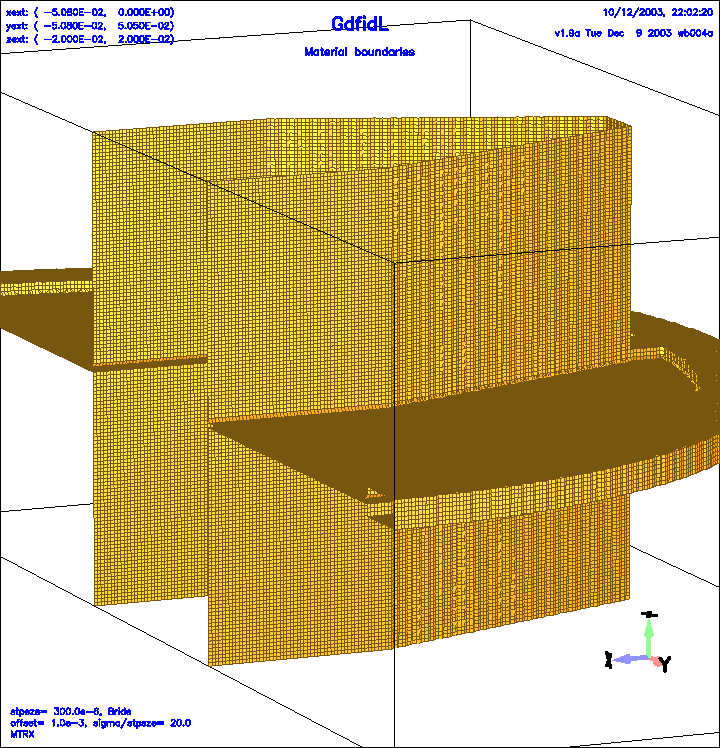
Figure 1:
The model of the flange (DSF1=1).
 |
The wakepotentials are computed when you perform a time domain computation with
a relativistic line charge as excitation.
The relevant part of such an inputfile is:
 -fdtd
    -ports
       name= beamlow,  plane= zlow,  modes= 0, npml= 30, doit
       name= beamhigh, plane= zhigh, modes= 0, npml= 30, doit
    -lcharge
       charge= 1e-12
       sigma= SIGMA       # Your sigma
       xposition= 0
       yposition= OFFSET  # The y-offset of the relativist line charge
       shigh= 6   # Perform a long range wakepotential computation.
We start the computation of the time dependet fields with the command:
single.d1 -host=ALL < flange0.gdf | tee out
The parameter -host=ALL tells single.gd1 to perform the computation in parallel
on all processors that are specified in the parallel virtual machine.
The computation will take some hours on a single CPU of a 2003 workstation.
The inputfile for this flange is
flange0.gdf
We start the postprocessor to compute the wakepotentials and impedance from the data
which were recorded during the time domain computation.
We start the postprocessor, gd1.pp, and use him interactively:
Input for gd1.pp:
     -general, infile= @last

     -wakes
        impedance= yes
        doit
 -------
 Thats it.
When we change the parameter DS1 in the inputfile, we are changing the
gap width of the flange. We will now study how the impedance depends on
that gap width.
Figure 2:
Flange with DSF1=1.
The transverse impedance in y-direction.
We observe that the potential seems not to decay at all.
We may therefore assume that the potential for larger s-values
consists purely of some linear combination of periodic functions.
The period length of these functions is given by the resonant frequencies
of resonant fields of the structure.
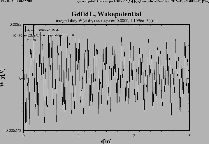 |
Figure 3:
Flange with DSF1=1.
The real part of the transverse impedance in y-direction.
We observe four large peaks, and some smaller ones.
The large peaks are near f=1.8GHz, f=5.5GHz and f=9.8GHz.
This impedance was computed from a wakepotential up to s=3 meters.
If the wakepotential eg. up to 10 meters would have been used,
the sharp peaks would become even high, but more narrow.
These sharp peaks correspond to modes which do not
couple at all or do not couple good to the beampipe,
but nevertheless have a substantial shunt-impedance.
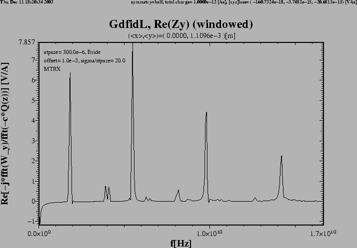 |
Figure 4:
Flange with DSF1=3.
The real part of the transverse impedance in y-direction.
The impedance is very similiar to the impedance of the flange
with DSF1=1, ie. the position of the peaks in the impedance
does not depende strongly on the gap width of the flange.
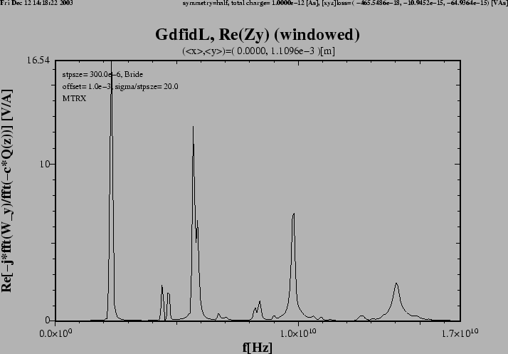 |
Figure 5:
Flange with DSF1=30.
This is a flange with a quite large gap, much larger than one would
have in practice.
The real part of the transverse impedance in y-direction.
We still observe some large peaks, and some broader ones.
The peaks are near f=2.3GHz, f=5.3GHz and f=9.8GHz.
The sharp peaks again correspond to modes which do not
couple at all or do not couple good to the beampipe,
but nevertheless have a substantial shunt-impedance.
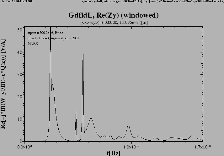 |
Figure 6:
The electric field in a geometry with DSF1=15.
The field was excited by a relativistic line charge traveling
near the line (x,y,z)=(0,0,z).
The linecharge was flying through the inhomogeneity at the time t=0.
The shown field exists at the time t=1.69 ns.
All energy which can escape through the beam pipes did already escape.
Only energy in modes with high Q-values is still in the computational
volume.
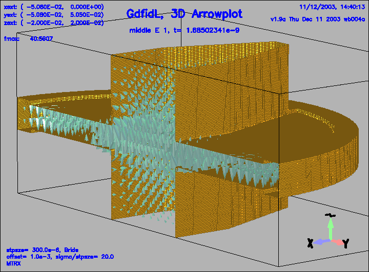 |
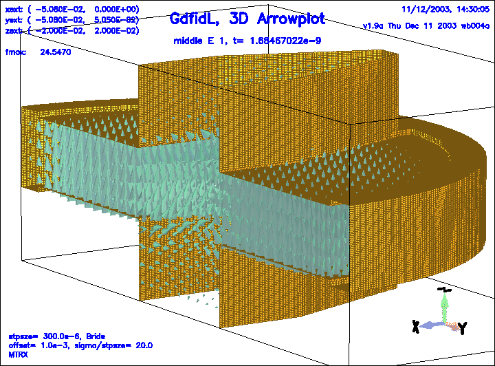
Figure 7:
The electric field in a geometry with DSF1=30.
All energy which can escape through the beam pipes did already escape.
 |
The structure itself is symmetric with respect to the plane z=0.
We model only half of the structure, the lower half, by specifying
pzhigh= 0, czhigh= electric.
The lower border of the computational volume is specified as a magnetic wall.
The computed resonant frequencies of the first 10 resonant modes in a structure
where the condition at the lower plane of the computational volume (in the beampipe)
is a magnetic wall, are 1.77, 1.83,, 3.9, 4.1, 4.4, 5.5, 5.6, 6.3, 6.5, and 6.7 GHz.
Figure 8:
A resonant field, electric field in a geometry with DSF1=1.
This is the field pattern of the mode with the lowest frequency, f=1.77 GHz.
That frequency is shown on the plot.
This resonance can not couple to the beampipe, since its frequency is lower than
the cutoff frequency of the beampipe.
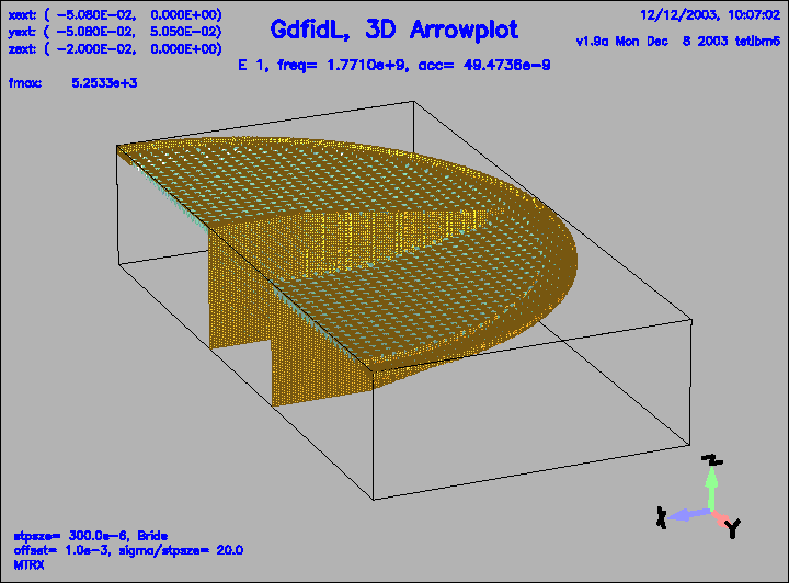 |
Figure 9:
The magnetic field of the first eigenfield.
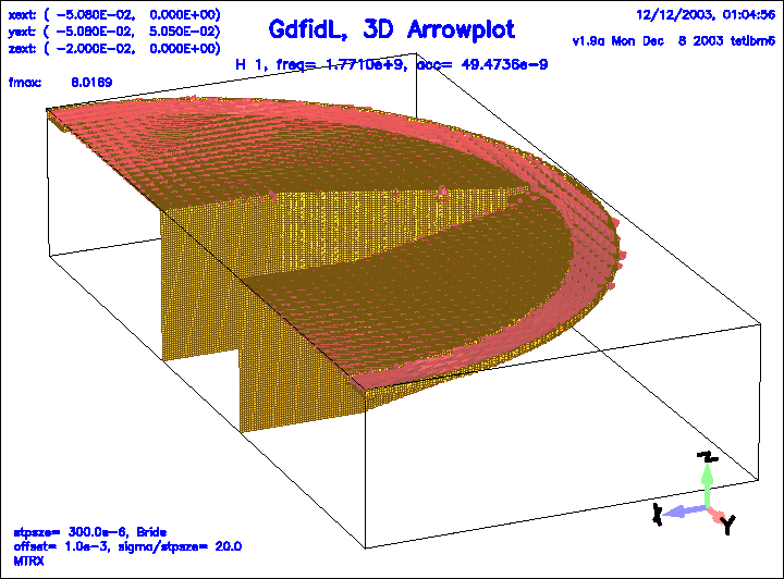 |
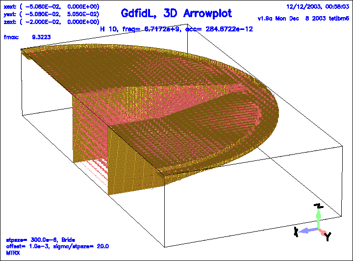
Figure 10:
The electric field of the second eigenfield, f=1.8 GHz.
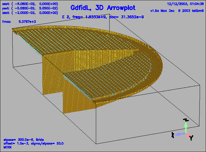 |
Figure 11:
The magnetic field of the second eigenfield.
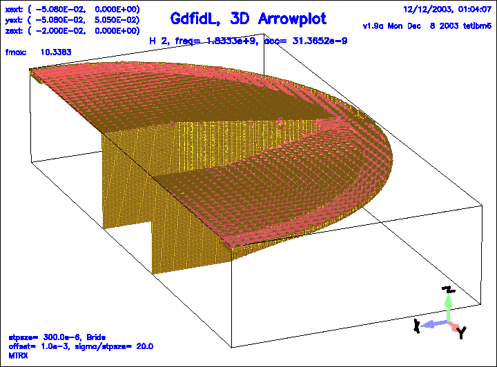 |
Figure 12:
The electric field of the 3.rd eigenfield.
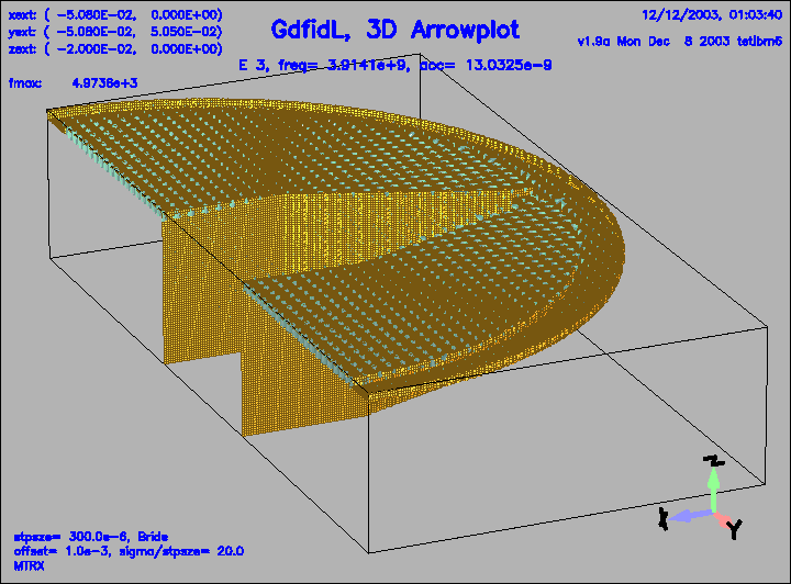 |
Figure 13:
The magnetic field of the 3.rd eigenfield.
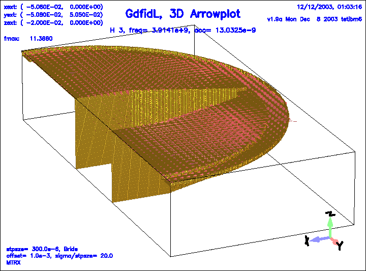 |
Figure 14:
The electric field of the 4.th eigenfield.
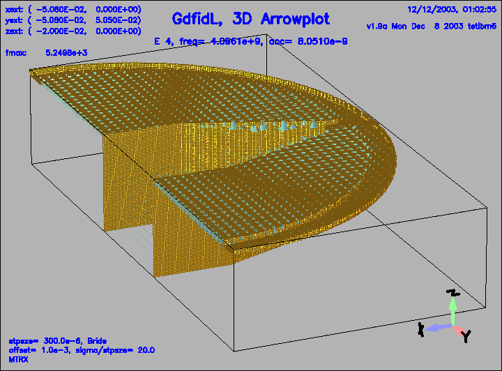 |
Figure 15:
The magnetic field of the 4.th eigenfield.
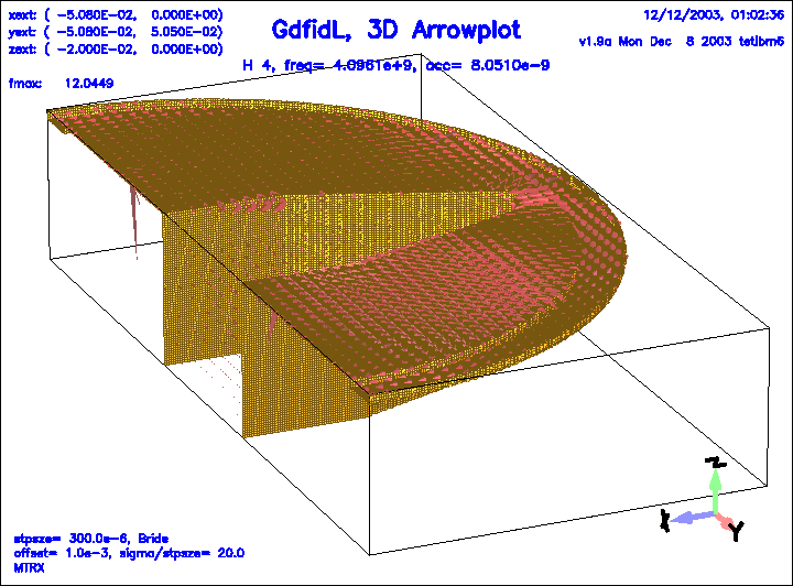 |
Figure 16:
The electric field of the 5.th eigenfield.
This field is coupled quite strong to the pipe.
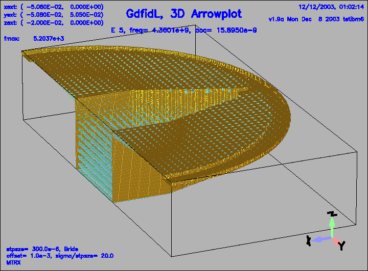 |
Figure 17:
The magnetic field of the 5.th eigenfield.
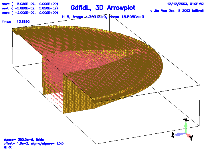 |
Figure 18:
The electric field of the 6.th eigenfield.
This field is weakly coupled to the pipe.
 |
Figure 19:
The magnetic field of the 6.th eigenfield.
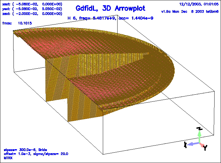 |
Figure 20:
The electric field of the 7.th eigenfield.
This field is weakly coupled to the pipe.
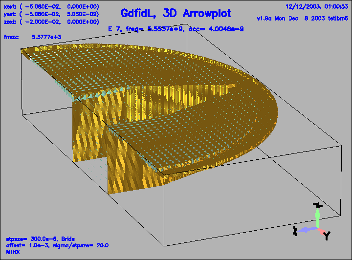 |
Figure 21:
The magnetic field of the 7.th eigenfield.
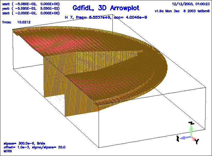 |
Figure 22:
The electric field of the 8.th eigenfield.
This field is weakly coupled to the pipe.
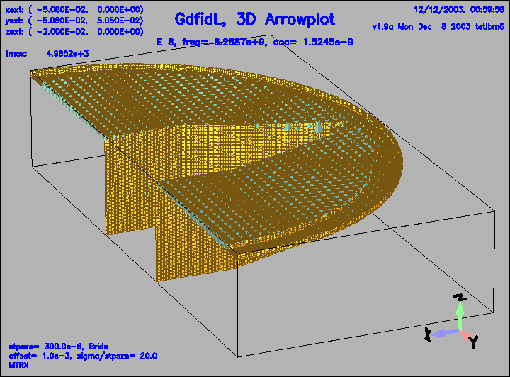 |
Figure 23:
The magnetic field of the 8.th eigenfield.
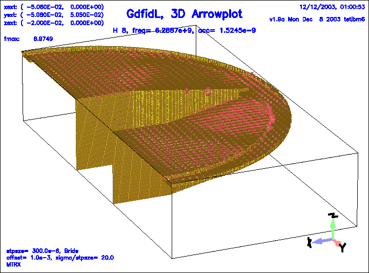 |
Figure 24:
The electric field of the 9.th eigenfield.
This field is weakly coupled to the pipe.
 |
Figure 25:
The magnetic field of the 9.th eigenfield.
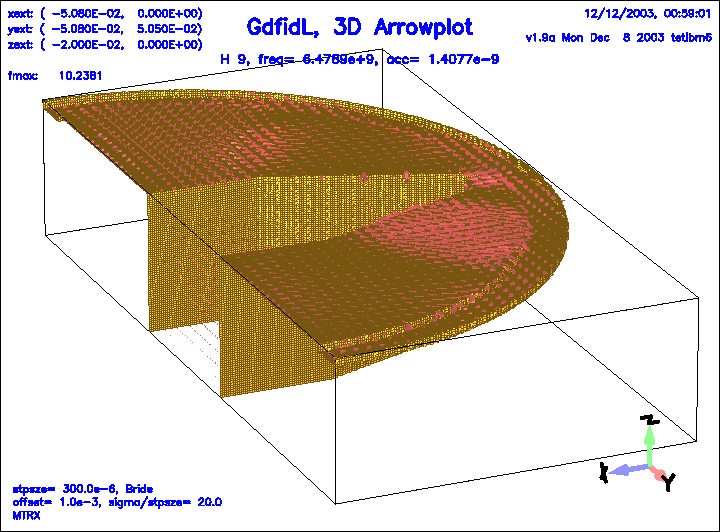 |
Figure 26:
The electric field of the 10.th eigenfield.
This field is coupled strong to the pipe.
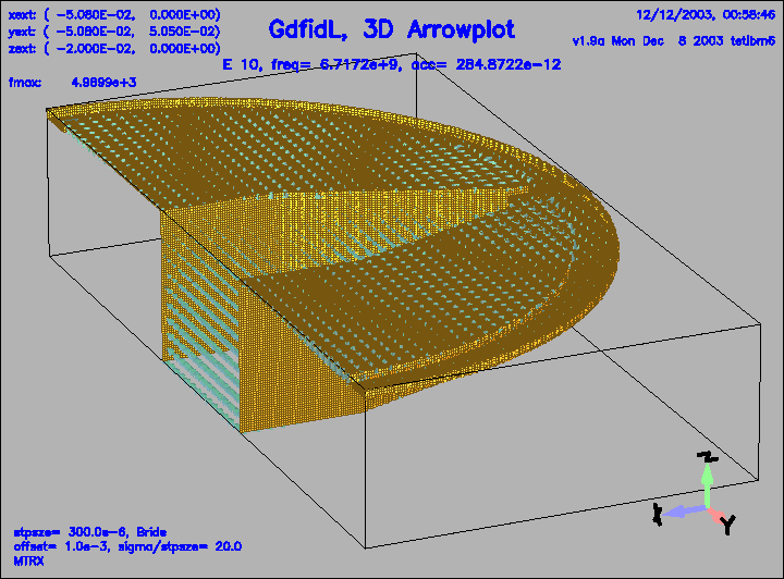 |
Figure 27:
The magnetic field of the 10.th eigenfield.
 |