-3darrowplot: Plots 3D Fields together with the material boundaries.

 ##############################################################################
 # Flags: nomenu, noprompt, nomessage,                                        #
 ##############################################################################
 # section: -3darrowplot                                                      #
 ##############################################################################
 # symbol      = e_1                                                          #
 # quantity    = e                                                            #
 # solution    = 1                                                            #
 # component   = all                    -- (x|y|z|all)                        #
 #    phase    = 45.0                   -- only for portmodes                 #
 # arrows      = 10000                                                        #
 # lenarrows   = 2.0                                                          #
 # maxlenarrows= 2.0                                                          #
 #   fcolour   =  4                                                           #
 # materials   = yes                    -- (yes | no)                         #
 # dielectrics = yes                    -- (yes | no)                         #
 # fonmaterials= no                     -- (yes | no)                         #
 #    logfonmat= no                     -- (yes | no)                         #
 #    fmaxonmat= auto                                                         #
 # scale       = 2.80                                                         #
 # fscale      = auto                                                         #
 # nlscale     = no , nlexp= 0.30                                             #
 # eyeposition = ( -1.0, -2.30, 0.50 )                                        #
 # bbxlow =    -1.0000e+30, bbylow =    -1.0000e+30, bbzlow =    -1.0000e+30  #
 # bbxhigh=     1.0000e+30, bbyhigh=     1.0000e+30, bbzhigh=     1.0000e+30  #
 # rotx   =     0.0000    , roty   =     0.0000    , rotz   =     0.0000      #
 # clouds = yes     -- show clouds                                            #
 ##############################################################################
 # plotopts     = -geometry 690x560+10+10                                     #
 # showtext     = yes                   -- (yes | no)                         #
 # showlines    = no                    -- (yes | no)                         #
 # onlyplotfiles= no                    -- (yes | no)                         #
 ##############################################################################
 # doit, ?, return, end, help, ls                                             #
 ##############################################################################

• symbol= QUAN_ISOL:
  This is the full name of the symbol to be processed.
• quantity= QUAN:
  This is the first part of the "symbol".
• solution= ISOL:
  This is the last part of the "symbol", the index of the "symbol".

• component:
  Possible values are x,y,z,all. Only the selected component will be plotted.
• phase:
  This parameter is used only when you want to plot the fields of portmodes. This specifies the phase of the phasor to be shown.
• arrows:
  The arrows that make up the plot are distributed equidistant over the whole computational volume. The number of points where an arrow is possible is given here.
• lenarrows:
  The relative length of the arrows that make up the plot. If lenarrows= 1, the arrows are scaled such, that for an homogeneous field the end of one arrow is just behind the end of the next arrow.
• maxlenarrows:
  No arrow shall be larger than this value.
  This is useful for fields where a strong field concentration happens, e.g. wakefields.
• fcolour= :
  The colour number of the field arrows.
• materials= :
  When yes, the material boundaries are plotted together with the fields.
• dielectrics= :
  When dielectrics= no, material boundaries between dielectrics will not be shown.
• fonmaterials= :
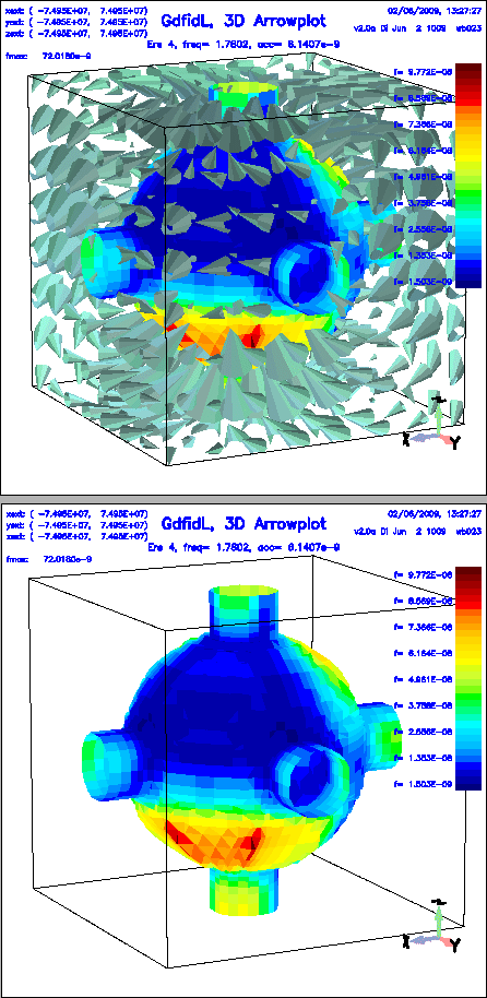
  A flag that specifies whether the colours of materialboundaries shall be encoding the field values near these material boundaries.
• logfonmat= :
  A flag that specifies whether the colours shall be assigned proportional to the logarithmic of the field value.
• maxfonmat= :
  What value shall be used as the largest field on the material patches. No further scaling takes place. This is useful for generating movies, where every frame of the movie should have the same colour encoding.
• scale= SCALE:
  The initial zoom factor of the resulting plot.
• fscale:
  If a value $\ne$ auto is specified, the vectorfield is scaled by this value. No further scaling takes place. This is useful for generating movies, where every frame of the movie should be scaled by the same factor.
• nlscale, nlexp:
  If nlscale= yes, the size of field arrows are proportional to the amplitude of the field to the power of nlexp.
• eyeposition= (XEYE, YEYE, ZEYE):
  This specifies the initial eyeposition for the 3D plot that will be produced. As soon as the plot appears, you can interactively change the eyeposition with the buttons of gd1.3dplot, but for a complex geometry, this may take some time.

• bbxlow=,bbxhigh=,bbylow=bbyhigh=,bbzlow=,bbzhigh=:
  Specifies the coordinates of a bounding box. Only the material-boundaries and the field-arrows that lie within the box are plotted.
• rotx= PhiX, roty= PhiY, rotz= PhiZ:
  This specifies the parameters of an additional rotation matrix. The data is rotated around the x-axis by an angle of PhiX, then the result is rotated around the y-axis by an angle of PhiY, and finally the result is rotated around the z-axis by an angle of PhiZ.

• clouds= :
  Selects, whether the position free moving charges shall be plotted together with the field.
• plotopts= ANY STRING CONTAING OPTIONS FOR THE PLOT-PROGRAMS:
  gd1.pp does not display the data itself, but writes a datafile for mymtv2 (1D and 2D data) or gd1.3dplot (3D data) and starts mymtv2 or gd1.3dplot to display these data.
  Useful options are:
  • -geometry X11-GEOMETRY Initial geometry for the X11 window of mymtv2 or gd1.3dplot.

• showtext= [yes|no]:
  This flags, whether the annotation text shall appear in the plots.

• showlines= :
  If yes, thin lines are plotted around the material patches, indicating the used discretisation.
• onlyplotfiles= [yes|no]:
  This flags, whether plotfiles shall be written AND mymtv2 or gd1.3dplot shall be started to display them on an X11 display, or whether only the plotfiles shall be produced.

Example To generate a plot of the first electric field found in the database, we say:

   symbol= e_1
   doit

Example To generate a plot of the real part of the fourth complex electric field found in the database, with the colours of the material patches showing the field strength at the material boundaries, we say:

   symbol= ere_4
   fonmat= yes
   doit

 # only the material plot, without the field:
 lena 1e-6
   doit

Figure 2.1: Above: Resulting plot, with field arrows, and material patches coloured according to the field strength at material boundaries. Below: The same plot, without field arrows.