Wake Potentials

The computation of wakepotentials occurs in two steps.

• gd1 is used to perform a time-domain computation with an exciting charge.
• Then gd1.pp is used to compute the wakepotentials from data that were recorded by gd1.

As a simple example, we use very strange geometry where we want to compute the wakepotentials of. The input for gd1 is

 # /usr/local/gd1/examples-from-the-manual/wake-example-1.gdf

define(LargeNumber, 1000)
#
# The following picture shows a cut through the structure to be
# modelled and the variables associated to the lengths.
#
#
#                a               a               a
#        |<------------->|<-------------->|<----------->|
#
#                 -      ------------------
#                 ^      |                |
#               b |      |                |
#                 |      |                |
#        -----------------                ---------------  -
#        |                     beam                     |  |
#        |<-------------------------------------------->|  | d
#        |                                              |  |
#        ------------------------------------------------  -
#
#    x^
#    |-> z
#
 define( a, 1e-2 )
 define( b, 5e-3 )
 define( c, 5e-3 )
 define( d, 1e-2 )

 -general
    outfile= /tmp/UserName/wake-example
    scratch= /tmp/UserName/wake-example-scratch

    text()= A strange geometry,
    text()= it serves only as an example
    text()= for computing wake-potentials.

 -mesh
define(STPSZE, 3*a/60 )
    spacing= STPSZE
    perfectmesh= no

    pxlow= 0, pxhigh= c+b
    pylow= -STPSZE, pyhigh= d
    pzlow= 0, pzhigh= 3*a

    cxlow= ele, cxhigh= ele
    cylow= ele, cyhigh= ele
    czlow= ele, czhigh= ele

    #
    # We enforce a meshline at the position of the linecharge
    # by enforcing two meshplanes
    #
    xfixed(1, c/2, 0)
    yfixed(1, d/2, 0)

 -brick
    #
    # fill the universe with metal
    #
    material= 1
       volume= (-LargeNumber, LargeNumber,\
                -LargeNumber, LargeNumber,\
                -LargeNumber, LargeNumber)
    doit

    #
    # carve out the waveguide
    #
    mat 0
       xlow= 0, xhigh= c
       ylow= 0, yhigh= LargeNumber
       zlow= -LargeNumber, zhigh= LargeNumber
    doit

    #
    # Carve out the resonator box
    #
    mat 0
       xlow= 0, xhigh= c+b
       ylow= 0, yhigh= LargeNumber
       zlow= a, zhigh= 2*a
    doit

 -volumeplot
   eyepos= ( 1.0, 2.30, 0.5 )
   showlines= yes
   scale= 2.5
   doit

 -fdtd
    -ports
       name= zlow, plane= zlow, modes= 0, doit
       name= zhigh, plane= zhigh, modes= 0, doit

    -lcharge
       charge= 1   # 1 As
       sigma= 5e-3
       xposition= c/2
       yposition= d/2

 -fdtd
     doit

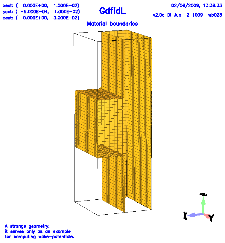
Figure 5.1: This volumeplot shows the discretised geometry. Although gd1 allows an inhomogeneous mesh even when a particle beam is present, this is not explicitely used here.

We start gd1 with the command:

   gd1 <  wake-example-1.gdf | tee out

The next step is to tell the postprocessor that we wish to see the wakepotentials: The commands for the postprocessor gd1.pp are:

 -general, infile= @last
 -wakes
    doit

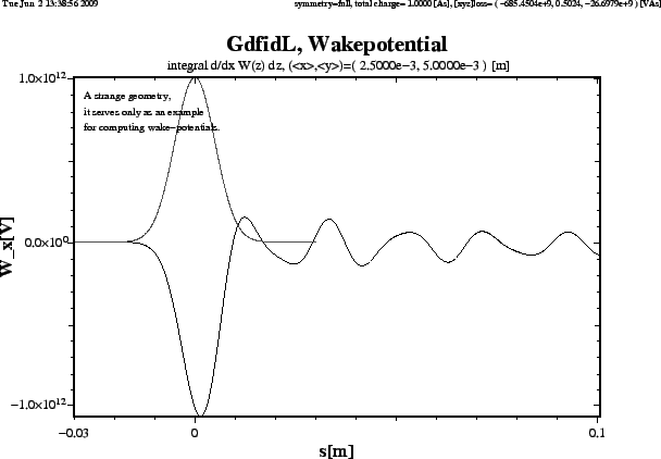
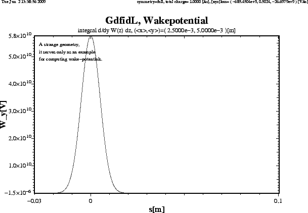
We get three plots for the three components of the wakepotential at the (x,y) coordinate where the line-charge was traveling.

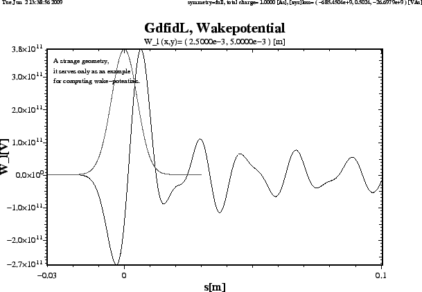
Figure 5.2: The z-component of the wakepotential at the (x,y)-coordinate where the exciting line charge was traveling. For reference, the shape of the exciting charge is plotted as well.

Figure 5.3: The two transverse components of the wakepotential at the (x,y)-coordinate where the exciting line charge was traveling. For reference, the shape of the exciting charge is plotted as well. The transverse wakepotentials are computed as the average of the transverse wakepotentials nearest to the coordinate where the line charge was traveling. The y-component of the wakepotential vanishes, as it should be.