Next: -material: Conductivities of electric Up: gd1.pp Previous: -clouds: Analyse properties of Contents

-sparameters: Computes scattering parameters from time dependent data

 ##############################################################################
 # Flags: nomenu, noprompt, nomessage,                                        #
 ##############################################################################
 # section -sparameter                                                        #
 ##############################################################################
 # ports      = all                                                           #
 #               -- (all | LIST )                                             #
 # modes      = ( 1 )                         -- (all | LIST )                #
 # timedata   = no                            -- ( yes | no )                 #
 #   tsumpower= no                            -- ( yes | no )                 #
 #   tintpower= no                            -- ( yes | no )                 #
 #   usample  = 5                             -- undersample for t-plots      #
 # freqdata   = yes                           -- ( yes | no )                 #
 #   wantdf   = auto                          -- ( auto | REAL )              #
 #   windowed = yes                           -- ( yes | no )                 #
 #     edgeofwindow = 0.70             -- at what frac. start to apply window #
 #   fsumpower= yes                           -- ( yes | no )                 #
 #   magnitude= yes                           -- ( yes | no )                 #
 #     slog   = no                            -- ( yes | no )                 #
 #   fintpower= no                            -- ( yes | no )                 #
 #   phase    = no                            -- ( yes | no )                 #
 #   smithplot= no                            -- ( yes | no )                 #
 #     markerat= undefined              -- want a marker at .. in smith-chart #
 #   groupvelocity= no                        -- ( yes | no )                 #
 #   fri      = no                            -- ( yes | no )                 #
 # excdata    = yes                     -- show the data of the excitation    #
 # upto       = auto                    -- [s]   ( auto | REAL )              #
 # flow       = auto                    -- [1/s] ( auto | REAL )              #
 # fhigh      = auto                    -- [1/s] ( auto | REAL )              #
 # ignoreexc  = no                            -- ( yes | no )                 #
 # details    = no                            -- ( yes | no )                 #
 ##############################################################################
 # plotopts = -geometry 690x560+10+10                                         #
 # showtext     = yes         -- (yes | no)                                   #
 # onlyplotfiles= no          -- (yes | no)                                   #
 ##############################################################################
 # return, help, end, ls, clearmarkers, doit                                  #
 ##############################################################################

ports:
Possible values are all, or a list of names of ports.
If ports= all, the time dependent data of all ports found in the data-base are processed.
If ports is a list of names, only the time dependent data of the ports whose names are found in the list are processed.
modes:
Possible values are all, or a list of mode-numbers.
If modes= all, the time dependent data of all modes of the selected ports found in the data-base are processed.
If modes is a list of mode-numbers, only the time dependent data of the modes with numbers in the list are processed.
timedata:
If timedata= yes, the time dependent amplitudes of the selected modes are plotted.
- tsumpower:
  If "yes", the sum of the power of the selected modes is computed as a function of time.
- tintpower:
  If "yes", the sum of the power of the selected modes is computed as a function of time and integrated over time.
- usample= NN:
  The undersampling factor to use for plots of time data.
freqdata:
If freqdata= no, no scattering parameters are plotted.
- wantdf= DF:
  The wanted frequency resolution of the computed scattering parameters. If wantdf=auto, the computed scattering parameters have a frequency resolution of just df = 1 / simulated time.
  If wantdf=DF , the time data are assumed to be zero outside of the FDTD-simulated time window. These zero-padded time signals within a time window of DT = 1 / DF are FFTed, giving an apparent frequency resolution of DF.
- windowed:
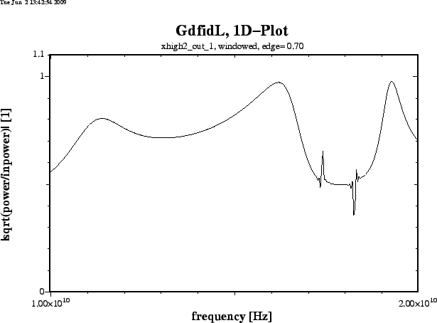
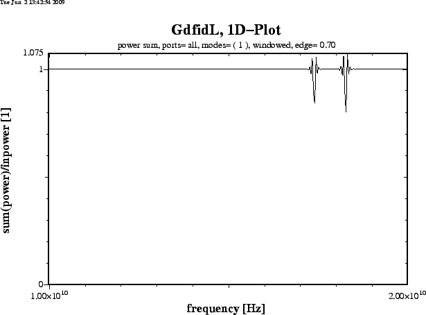
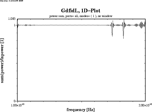
  If "yes", the time signals ar multiplied by a window-function, before FFTing them. This damps the ripples in the scattering parameters, when the impulse response is not yet fully computed.
- edgeofwindow= FRAC:
  The fraction of the simulated time, where the windowing function shall start to decay.
  The applied windowing function is a constant '1' from t=0 to FRAC * T, where T is the simulated time. After FRAC * T, the windowing function is
  
  $\begin{displaymath}\frac{1}{2} \left[1+\cos(\pi\frac{t-FRAC*T}{(1-FRAC)*T})\right] \end{displaymath}$
  
  .
- fsumpower:
  If "yes", the sum of the power of the selected modes as a function of frequency is computed and plotted.
- magnitude:
  If magnitude= yes, the absolute value of the scattering parameters are plotted.
- slog:
  If slog= yes, the magnitude of the scattering parameters are initially plotted in a logarithmic plot.
- fintpower:
  If "yes", the sum of the power of the selected modes as a function of frequency and integrated over frequency is computed and plotted.
- phase:
  If phase= yes, the phase of the scattering parameters are plotted.
- smithplot:
  If smithplot= yes, the scattering parameters are plotted in a smith-plot.
- markerat= Fi:
  Specifies that you want to have a marker near the frequency Fi in the smith plots. You may specify an unlimited number of frequencies where you want markers at.
- groupvelocity:
  If groupvelocity= yes, the groupvelocity is computed from the phase. The result only makes sense for transmissions.
- fri:
  If fri= yes, the scattering parameters are written in fri-format to files.
excdata:
Whether the data of the excitation shall be plotted.
upto:
Possible values are auto or a time-value.
If upto= auto, the time data upto the last found simulated time are considered for the fourier-transforms.
If upto= TMAX, only the time-data upto the time-value TMAX are considered for the fourier-transforms. This is useful, for the case that a late time instability of the time domain computation has occured, and you want to know the scattering parameters of a shorter simulation. THIS SHOULD NOT HAPPEN. IF YOU ENCOUNTER A LATE TIME INSTABILITY, PLEASE SEND THE INPUTFILE WHERE THIS INSTABILITY HAS OCCURED TO "bruns@gdfidl.de".
--
If "upto" is specified as a value larger than the time simulated by the FDTD-solver, then the time values up to "upto" are filled up with zeroes. This has the effect that additional frequency points are computed by FFTing the padded data set. The scattering parameters at the additional frequency points are interpolated from the primary frequency dependent values by a sin(x)/x interpolation. For such a purpose, you should better specify wantdf= DF.
flow:
If flow= auto, the lower boundary of the frequency range of the plots is derived from the centerfrequency and the bandwidth of the excitation as they were specified in the input for gd1. If flow= FMIN, the lower boundary of the frequency range is FMIN.
fhigh:
If fhigh= auto, the upper boundary of the frequency range of the plots is derived from the centerfrequency and the bandwidth of the excitation as they were specified in the input for gd1. If fhigh= FMAX, the lower boundary of the frequency range is FMAX.
ignoreexc:
If ignoreexc= yes, the spectrum of the excited mode is ignored. Instead a flat spectrum is assumed. This is useful e.g. to compute the coupling from an relativistic charge to the port-modes.
details:
If yes, a lot of intermediate results are plotted.
doit:
The scattering parameters are computed from the time dependent amplitudes of the port-modes.
clearmarkers:
If you say clearmarkers, the list of markers which were requested via markerat is cleared.

Example To compute and plot the scattering parameters of only the first two modes of the ports with names Input, Output, we say:

 -sparamater
     modes= ( 1, 2 )
     ports= ( Input, Output )
  doit

Example In the first step, we compute the time dependent amplitudes with gd1:

 gd1 < /usr/local/gd1/examples-from-the-manual/arndt.MTT90.p1854.fig5.gdf

In the next step, we start gd1.pp to compute the scattering parameters from the time dependent amplitudes, that were computed by gd1. The input we give to gd1.pp is:

 -gen, inf @last
 -3da, sy e_1, scal 4.5, arr 5000, doit
 -spa, window yes, doit
       window no, doit

The resulting plots are shown in the figures 2.2 to 2.12.

**Figure 2.2:** The time dependent electric field at an early time.
$\begin{figure}\epsfig{figure=/tmp/bruw1931/ps-Files/arndt.MTT90.p1854.fig5.ps,width=18cm,bbllx=0pt,bblly=0pt,bburx=747pt,bbury=554pt,clip=}\end{figure}$

**Figure 2.3:** The computed reflection when a window has been applied.
$\begin{figure}\epsfig{figure=/tmp/bruw1931/ps-Files/arndt-res-window-xlow1_out_1... ...bs.ps,width=15cm,bbllx=0pt,bblly=43pt,bburx=776pt,bbury=575pt,clip=}\end{figure}$

**Figure 2.4:** A computed transmission when a window has been applied.
$\begin{figure}\epsfig{figure=/tmp/bruw1931/ps-Files/arndt-res-window-xlow2_out_1... ...bs.ps,width=15cm,bbllx=0pt,bblly=43pt,bburx=776pt,bbury=575pt,clip=}\end{figure}$

**Figure 2.5:** A computed transmission when a window has been applied.
$\begin{figure}\epsfig{figure=/tmp/bruw1931/ps-Files/arndt-res-window-xhigh1_out_... ...bs.ps,width=15cm,bbllx=0pt,bblly=43pt,bburx=776pt,bbury=575pt,clip=}\end{figure}$

**Figure 2.6:** A computed transmission when a window has been applied.
$\begin{figure}\epsfig{figure=/tmp/bruw1931/ps-Files/arndt-res-window-xhigh2_out_... ...bs.ps,width=15cm,bbllx=0pt,bblly=43pt,bburx=776pt,bbury=575pt,clip=}\end{figure}$

**Figure 2.7:** The computed reflection when no window has been applied.
$\begin{figure}\epsfig{figure=/tmp/bruw1931/ps-Files/arndt-res-nowindow-xlow1_out... ...bs.ps,width=15cm,bbllx=0pt,bblly=43pt,bburx=776pt,bbury=575pt,clip=}\end{figure}$

**Figure 2.8:** A computed transmission when no window has been applied.
$\begin{figure}\epsfig{figure=/tmp/bruw1931/ps-Files/arndt-res-nowindow-xlow2_out... ...bs.ps,width=15cm,bbllx=0pt,bblly=43pt,bburx=776pt,bbury=575pt,clip=}\end{figure}$

**Figure 2.9:** A computed transmission when no window has been applied.
$\begin{figure}\epsfig{figure=/tmp/bruw1931/ps-Files/arndt-res-nowindow-xhigh1_ou... ...bs.ps,width=15cm,bbllx=0pt,bblly=43pt,bburx=776pt,bbury=575pt,clip=}\end{figure}$

**Figure 2.10:** A computed transmission when no window has been applied.
$\begin{figure}\epsfig{figure=/tmp/bruw1931/ps-Files/arndt-res-nowindow-xhigh2_ou... ...bs.ps,width=15cm,bbllx=0pt,bblly=43pt,bburx=776pt,bbury=575pt,clip=}\end{figure}$

**Figure 2.11:** The sums of the squares of the computes scattering parameters when a window has been applied.
$\begin{figure}\epsfig{figure=/tmp/bruw1931/ps-Files/arndt-res-window-sum-power-freq.ps,width=15cm,bbllx=0pt,bblly=43pt,bburx=776pt,bbury=575pt,clip=}\end{figure}$

**Figure 2.12:** The sums of the squares of the computes scattering parameters when no window has been applied.
$\begin{figure}\epsfig{figure=/tmp/bruw1931/ps-Files/arndt-res-nowindow-sum-power-freq.ps,width=15cm,bbllx=0pt,bblly=43pt,bburx=776pt,bbury=575pt,clip=}\end{figure}$

Next: -material: Conductivities of electric Up: gd1.pp Previous: -clouds: Analyse properties of Contents