Looking at the wakepotentials

We enter the section -wakes. When we are solely interested in the longitudinal and transverse wakepotentials at the position of the line-charge, we do not have to specify any special option, the default values are good for that. The default is to compute and plot the longitudinal and transverse wakepotentials at the position of the exciting charge. We say

 -wakes
     doit

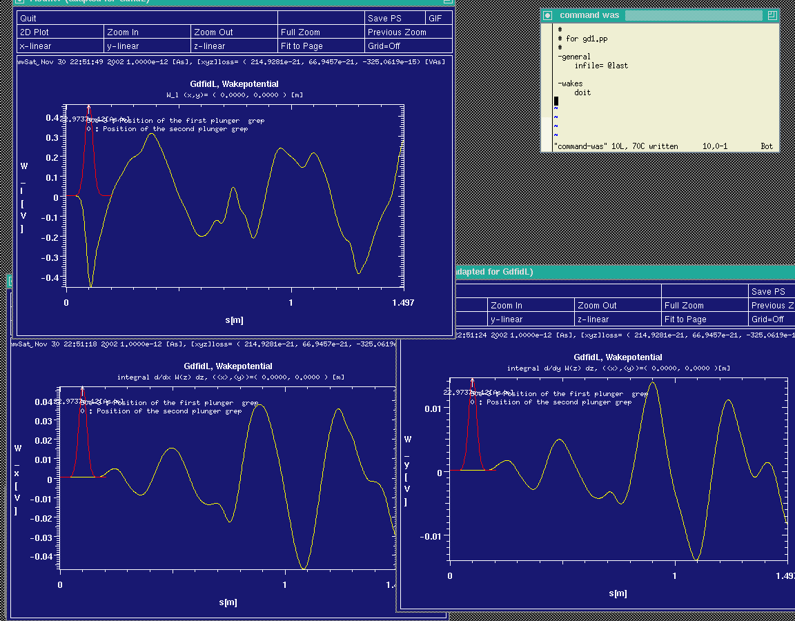
The resulting plots are shown in figure 10.4.

Figure 10.4: Screenshot of the desktop when we just said 'doit' in the section '-wakes'. gd1.pp has popped up three instances of mymtv2 that show the longitudinal and transverse wakepotentials at the (x,y) position of the line-charge. The yellow curves are the wakepotentials, and the red curve is the charge density of the line-charge.

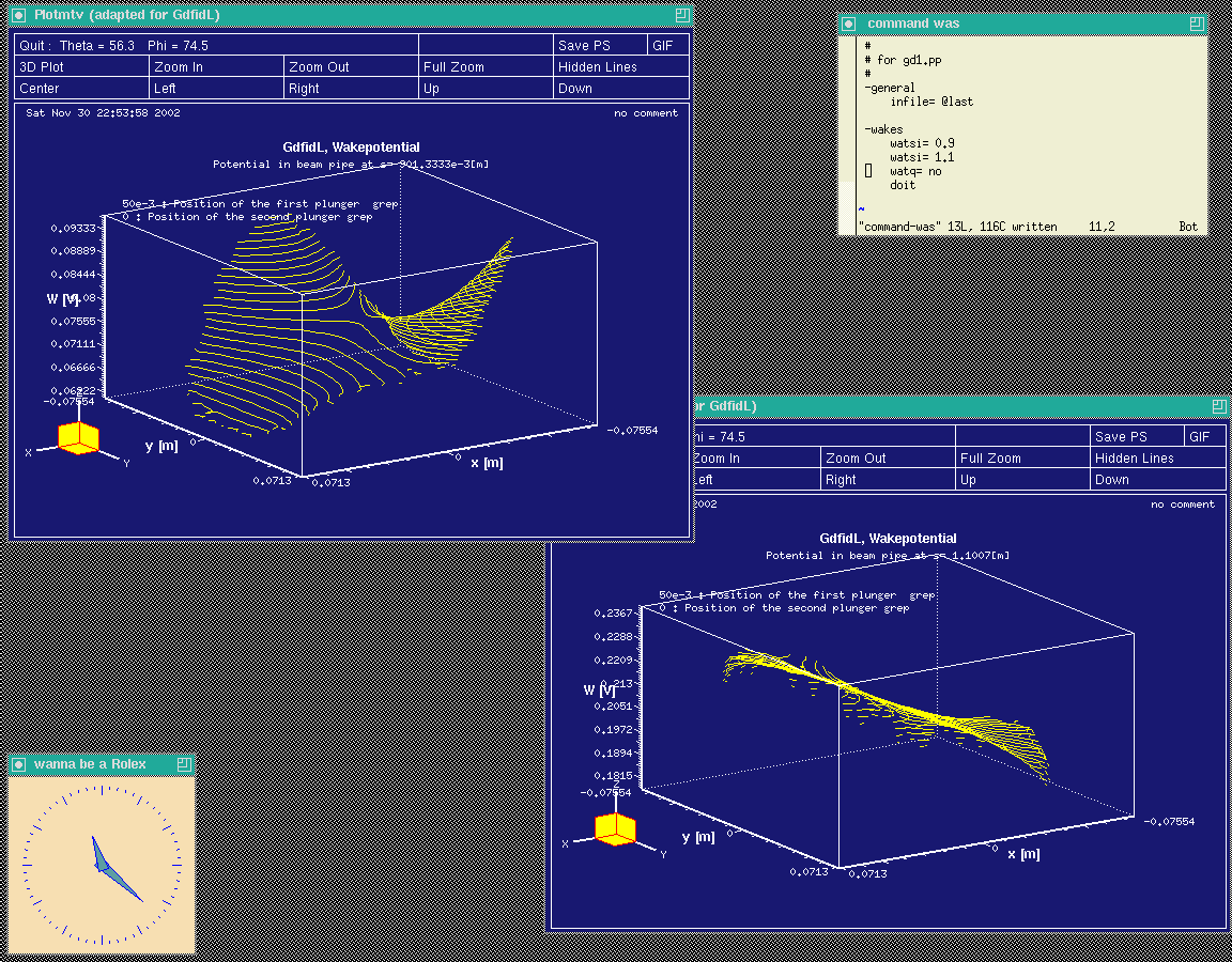
We look at the longitudinal wakepotential as a function of (x,y) at the s-positions s=0.9m and s=1.1m by specifying

 watsi= 0.9
 watsi= 1.1
 watq= no
 doit

the watq= no instructs gd1.pp that we do not want to see again the wakepotentials at the position of the linecharge. We did specify watsi= ?? twice, this means, that we want to see the wakepotential at both s-coordinates. The resulting plots are shown in figure 10.5.

Figure 10.5: Screenshot of the desktop showing the longitudinal wakepotential in the cross section of the beam-pipe where a beam can travel.