How to analyse the Doris cavity of the SRRC with GdfidL v1

Warner Bruns

December 1, 2002

$\psfig{figure=doris.perfect.PS,width=12cm,bbllx=28pt,bblly=74pt,bburx=571pt,bbury=792pt,clip=}$

List of Figures

Screenshot of a typical desktop when one uses gd1. The xterm in the upper right corner is used to edit the inputfile, the xterm in the lower right is used to feed gd1 with the inputfile, and the long xterm on the right side runs another instance of gd1. This second instance of gd1 is used to look-up the syntax of gd1's command language.
A drawing of the main cavity.
Screenshot of the desktop when the inputfile doris00.gdf has been fed into gd1. gd1 has popped up an instance of mymtv2 that shows the outline of the specified polygon.
Screenshot of the desktop when the inputfile doris01.gdf has been fed into gd1. gd1 has popped up an instance of gd1.3dplot that shows the generated mesh.
Screenshot of the desktop when the inputfile doris02.gdf has been fed into gd1. gd1 has popped up an instance of gd1.3dplot that shows the generated mesh. We now have only the eighth part of the total structure.
Screenshot of the desktop. gd1.pp has popped up three instances of gd1.3dplot, showing the electric field of the first three modes.
Screenshot of the desktop. gd1.pp has popped up three instances of gd1.3dplot, showing the magnetic field of the first three modes.
component of the first mode on the axis x=y=0. Since only the part of the structure below the plane z=0 is modeled, we only have direct information about the field below z=0. Clearly, the -component is even with respect to the plane z=0.
The real part and imaginary part of the integrated voltage as a function of the position x. This plot has not been generated directly by gd1.pp, but has been produced by a simple shell-script.
Screenshot of the desktop when the default values in -wakes are used. The three instances of mymtv2 show the longitudinal and transverse wakepotentials at the position of the line charge, ie at the position (x,y)=(0,0). The yellow curves show the wakepotentials, the red curves show the used line-charge density. The upper left mymtv2 shows the longitudinal wakepotential, while the lower two mymtv2-windows show the transverse wakepotentials.
Screenshot of the desktop when the plots of wakes in a plane are requested. The two instances of mymtv2 show the longitudinal and transverse wakepotentials near the plane y=0.
The electric field as induced by a line charge traveling on the axis. The direction of the arrows indicate the direction of the field, and their size is proportional to the absolute value of the field strength.
The electric field as induced by a line charge traveling on the axis. The direction of the arrows indicate the direction of the field. Their size now is not proportional to the field strength, since we did specify that there should be a treshold value of "maxlenarrows= 2".
The technical drawing with the plungers, pumping hole and feeding loop.
Details of the technical drawing, showing the plungers.
An outline of the body of revolution that shall decribe the body of a plunger.
The plunger now has its axis showing in the right direction.
Screenshot of the desktop when the inputfile wPlunger00.gdf has been fed into gd1.
Screenshot of the desktop when the inputfile wPlunger01.gdf has been fed into gd1. Shown is a zoom of the interesting region near the plungers.
A plot of the real part and imaginary part of the accelerating voltage of the monopole mode in the cavity with plungers. Only the real part would be nonzero, if the symmetry plane at z=0 would not have been used. One can clearly see that the accelerating voltage no longer is independent of the x-position.
Screenshot of the desktop showing the matrialdistribution and the wakefield at some time. We cannot see the wakefield, since the material boundaries hide the field.
Screenshot of the desktop when we switched off the plotting of the material-boundaries.
Screenshot of the desktop when we switched on the plotting of the material-boundaries, but selected bbzhigh=0.
Screenshot of the desktop when we just said 'doit' in the section '-wakes'. gd1.pp has popped up three instances of mymtv2 that show the longitudinal and transverse wakepotentials at the (x,y) position of the line-charge. The yellow curves are the wakepotentials, and the red curve is the charge density of the line-charge.
Screenshot of the desktop showing the longitudinal wakepotential in the cross section of the beam-pipe where a beam can travel.
Screenshot of the desktop showing the longitudinal and transverse wakepotential near the plane x=0.
Screenshot of the desktop showing the longitudinal and transverse wakepotential near the plane y=0.

What this paper contains

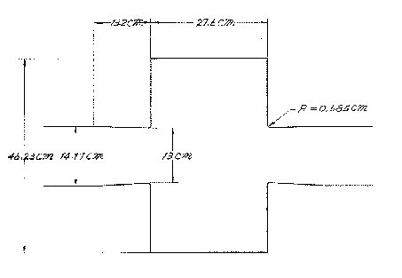
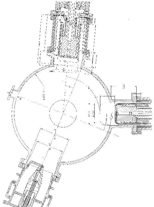
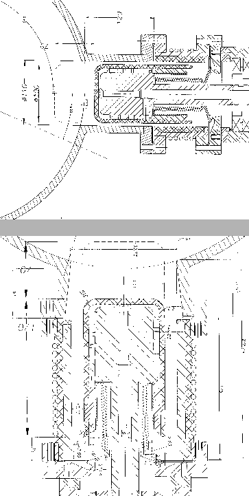
We got detailed technical drawings¹ of a Doris cavity.

The data from these drawings are transformed step by step into an inputfile for gd1. Every step is explained in detail. Numerous hints are given, how one effectively models ones geometry. When we have modelled the geometry accurately enough, we compute the fields and wakepotentials.

Analysing the rotational symmetric part of the cavity

Meshing

Recommended usage of gd1

The most effective usage of gd1 is:

Write an inputfile
Until gd1 does what you want him to do:
- feed gd1 with the inputfile
- Change the inputfile

If you work with several xterms, this cycle is very fast. Figure 1.1 shows a typical ``desktop`` with three xterms. The upper right xterm is a terminal running an editor to change the inputfile, the lower right xterm is used to feed gd1 with the actual inputfile, and a third xterm is used to run another instance of gd1. This second instance of gd1 is used to look-up the syntax of gd1's commands.

**Figure 1.1:** Screenshot of a typical desktop when one uses **gd1**. The xterm in the upper right corner is used to edit the inputfile, the xterm in the lower right is used to feed **gd1** with the inputfile, and the long xterm on the right side runs another instance of **gd1**. This second instance of **gd1** is used to look-up the syntax of **gd1**'s command language.
$\begin{figure}\begin{center}\psfig{figure=dumped00.PS,width=524pt} \end{center} \end{figure}$

Modelling the geometry

**Figure 1.2:** A drawing of the main cavity.
$\begin{figure}\centerline{ \psfig{figure=cavity01.PS,width=10cm} }\end{figure}$

The cavity we want to analyse is essentially a body of revolution. There are two plungers attached, that are presumably for tuning the cavity. In addition, a small tube is attached, that is probably used for maintaining the vacuum.

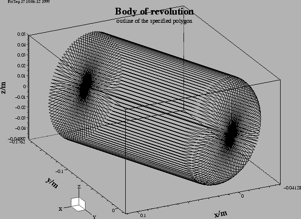
In the first step we model the cavity and the beam-pipes. We do this by specifying a polygonal description of the boundary in the r-z-plane. The inputfile that describes the boundary is:

 #
 # Some helpful symbols:
 #
 define(EL, 1) define(MAG, 2)
 define(INF, 1000)

 #
 # We define symbols that will be used to describe our cavity:
 # The names of the symbols can be up to 32 characters long,
 #
 define(OuterRadius   , 46.23e-2/2 )
 define(InnerRadius   , 13.00e-2/2 )
 define(GapLength     , 27.60e-2   )
 define(CurveRadius   ,  0.585e-2  )
 define(BeamPipeRadius, 14.17e-2/2 )
 define(TaperLength   , 13.2e-2    )

 -brick
     material= EL
     xlow= -INF, xhigh= INF
     ylow= -INF, yhigh= INF
     zlow= -INF, zhigh= INF
     doit
 
 #
 # we carve out the body of the cavity
 #

 -gbor
    material= 0
    origin= (0,0,0)
    zprimedirection= (0,0,1)
    rprimedirection= (1,0,0)
    range= (0,360)

    clear      # clear any old polygon-description
      # point= (z,r)
    point= ( -(GapLength/2+TaperLength+10e-2), 0              ) # p1
    point= ( -(GapLength/2+TaperLength+10e-2), BeamPipeRadius )
    point= ( -(GapLength/2+TaperLength      ), BeamPipeRadius )
    point= ( -(GapLength/2+CurveRadius      ), InnerRadius    )
      arc, radius= CurveRadius, size= small, type= counterclockwise
    point= ( -(GapLength/2                  ), InnerRadius+CurveRadius )
    point= ( -(GapLength/2                  ), OuterRadius    )
     ## crossing z=0 plane
    point= (  (GapLength/2                  ), OuterRadius    )
    point= (  (GapLength/2                  ), InnerRadius+CurveRadius )
      arc, radius= CurveRadius, size= small, type= counterclockwise
    point= (  (GapLength/2+CurveRadius      ), InnerRadius    )
    point= (  (GapLength/2+TaperLength      ), BeamPipeRadius )
    point= (  (GapLength/2+TaperLength+10e-2), BeamPipeRadius )
    point= (  (GapLength/2+TaperLength+10e-2), 0              )
 show= now
 doit

 -volumeplot
    doit

This inputfile can be found as "/usr/local/gd1/Tutorial-SRRC/doris00.gdf". When we feed this file into gd1 via the command "gd1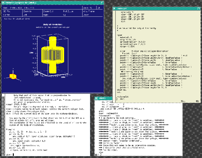

doris00.gdf", we get a desktop similiar to the one shown in figure 1.3

**Figure 1.3:** Screenshot of the desktop when the inputfile doris00.gdf has been fed into **gd1**. **gd1** has popped up an instance of **mymtv2** that shows the outline of the specified polygon.
$\begin{figure}\centerline{ \psfig{figure=doris00.PS,width=524pt} }\end{figure}$

gd1 does not what we want, we do not get a "volumeplot", although we requested one. But gd1 gives us a hint what we made wrong:

 volumeplot>     doit
 # I am checking the mesh settings..
   .. plane x= xlow  in "-mesh" is undefined..
   .. plane x= xhigh in "-mesh" is undefined..
   .. plane y= ylow  in "-mesh" is undefined..
   .. plane y= yhigh in "-mesh" is undefined..
   .. plane z= zlow  in "-mesh" is undefined..
   .. plane z= zhigh in "-mesh" is undefined..
 *** section -mesh: "spacing= undefined"..
 *** errors in "mesh"..
 *** Since this not seems to be an interactive session,
 *** I decide to treat this as a fatal error.
 *** Fix the input.
 stop

When we say "doit" in the section "-volumeplot", gd1 tries to generate the mesh. But in order to generate the mesh, gd1 needs to know

what the extreme coordinates of the computational volume shall be,
what the default mesh spacing shall be.

All these informations have to be given to gd1 before a volumeplot is requested. Since gd1 has detected that it is fed by an inputfile and is not used interactively, it stops as soon some essential information is not available. When not run interactively, gd1 also stops when some syntax error is present in the inputfile.

To give gd1 the needed information, we change our inputfile. We insert the following lines somewhere before "-volumeplot":

 ###
 ### We define the borders of the computational volume,
 ### and we define the default mesh-spacing.
 ###
 -mesh
     spacing= InnerRadius/15
     pxlow= -1.1*OuterRadius, pxhigh= 1.1*OuterRadius
     pylow= -1.1*OuterRadius, pyhigh= 1.1*OuterRadius
     pzlow = -(GapLength/2+TaperLength+9e-2)
     pzhigh= +(GapLength/2+TaperLength+9e-2)

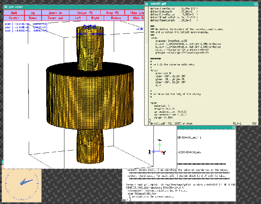
The so edited inputfile can be found as "/usr/local/gd1/Tutorial-SRRC/doris01.gdf".

When we feed gd1 with this inputfile (gd1 doris01.gdf) we get a screen similiar to the one shown in figure 1.4

**Figure 1.4:** Screenshot of the desktop when the inputfile doris01.gdf has been fed into **gd1**. **gd1** has popped up an instance of gd1.3dplot that shows the generated mesh.
$\begin{figure}\centerline{ \psfig{figure=doris01.PS,width=524pt} }\end{figure}$

Enforcing Meshplanes

For bodies of revolution, gd1 has no algorithm to decide where to place the meshplanes. We have to give gd1 a hint. We want to have meshplanes exactly at the bottom and the top of our cavity. We specify the wanted locations of the meshplanes in the section -mesh. We edit our inputfile so that it contains

   -mesh
      #
      # enforce two meshplanes, at the bottom and the top of the cavity:
      #
      zfixed(2, -GapLength/2, GapLength/2 )

The semantics of zfixed(N, Z0, Z1) is: N is the number of meshplanes to enforce, the meshplanes are placed equidistantly between Z0 and Z1. It is allowed to specify positions of mesh-planes that are outside of the computational volume.

Since we have had already a quite fine mesh, the effect is not visible and is not shown here.

There is not much gain if one tries to enforce meshplanes at the outer radii of the cavity and the beam-pipes.

Symmetry Planes

We now have our main cavity discretised. In principle, we could now compute the resonant fields in it. But we better use the symmetries of the cavity. We have three symmetry planes: The cavity is symmetric with respect to the plane z=0, and to the plane x=0 and to the plane y=0.

We specify that we only want to compute in the volume $x \le 0, y \le 0, z \le 0$ by specifying the borders of the computational volume accordingly. We change the specifications in the inputfile to

 ###
 ### We define the borders of the computational volume,
 ### and we define the default mesh-spacing.
 ###
 -mesh
     spacing= InnerRadius/15
     pxlow= -1.1*OuterRadius
     pylow= -1.1*OuterRadius
     pzlow = -(GapLength/2+TaperLength+9e-2)
     pxhigh= 0
     pyhigh= 0
     pzhigh= 0

When we feed gd1 with this inputfile (gd1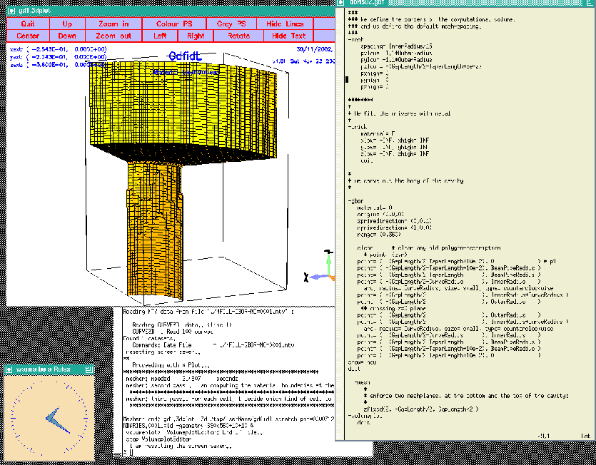

doris02.gdf) we get a screen similiar to the one shown in figure 1.5

**Figure 1.5:** Screenshot of the desktop when the inputfile doris02.gdf has been fed into **gd1**. **gd1** has popped up an instance of gd1.3dplot that shows the generated mesh. We now have only the eighth part of the total structure.
$\begin{figure}\centerline{ \psfig{figure=doris02.PS,width=524pt} }\end{figure}$

Boundary conditions

Now that we have taken care of the symmetry planes, we have to specify the boundary conditions at these planes. We have to tell gd1 what conditions are to be applied at the six planes x=xlow, x=xhigh, y=ylow, y=yhigh, z=zlow, z=zhigh. The possible values are: electric boundary conditions, magnetic boundary conditions, and periodic boundary conditions. For our problem, we only need electric and magnetic boundary conditions. We specify these conditions again in the section "-mesh". We edit our inputfile such that the entries for -mesh now look like:

 ###
 ### We define the borders of the computational volume,
 ### we define the default mesh-spacing,
 ### and we define the conditions at the borders:
 ###
 -mesh
     spacing= InnerRadius/15
     pxlow= -1.1*OuterRadius
     pylow= -1.1*OuterRadius
     pzlow = -(GapLength/2+TaperLength+9e-2)
     pxhigh= 0
     pyhigh= 0
     pzhigh= 0

     #
     # The conditions to use at the borders of the computational volume:
     #
     cxlow= electric, cxhigh= magnetic
     cylow= electric, cyhigh= magnetic
     czlow= electric, czhigh= electric

We are not done yet: Since gd1 can compute resonant fields and time dependent fields, we have to specify what kind of field we are interested in. We want to compute resonant fields, so we specify this by entering at the end of our inputfile:

 -eigenvalues
    solutions= 15      # we want to compute with 15 basis vectors
    estimation= 10e9   # the estimated highest frequency
    doit

When we feed gd1 with this inputfile (gd1

doris03.gdf), gd1 complains about an IO-error:

 *** A component of the path prefix does not exist or the Path parameter points
 *** to an empty string.
 CreateDirectory: cmd: mkdir /tmp/--username--/--SomeDirectory--/Results
  error code: 2
 ** cannot open catalogue: iostat: 14
 ** catalogue: "/tmp/--username--/--SomeDirectory--/Results/catalogue"
 ** error msg: "No such file or directory / permission denied"
 InitializeDatabase: cannot read catalogue.. iostat: 14
 *** check "outfile" in section "-general"..
 *** errors in settings
 *** Since this not seems to be an interactive session,
 *** I decide to treat this as a fatal error.
 *** Fix the input.
 stop

We have not yet specified where the results of your computation shall be written to! We do this by editing our inputfile:

 ###
 ### We enter the section "-general"
 ### Here we define the name of the database where the
 ### results of the computation shall be written to.
 ###    (outfile= )
 ### We also define what names shall be used for scratchfiles.
 ###     (scratchbase= )
 ###
 -general
    outfile= /tmp/UserName/doris
    scratchbase= /tmp/UserName/doris-scratch

Summary

You have to give gd1 the following information:

what geometry you are interested in (-brick -gbor etc),
what the boundary planes of your computational volume are (-mesh),
what the conditions at these boundary planes are (-mesh),
what the default mesh density shall be (-mesh),
where gd1 shall store the result (-general),
what kind of computation gd1 shall perform (-eigenvalues, -fdtd).

The complete inputfile up to now (doris04.gdf) is:

 #
 # Some helpful symbols:
 #
 define(EL, 1) define(MAG, 2)
 define(INF, 1000)

 #
 # We define symbols that will be used to describe our cavity:
 # The names of the symbols can be up to 32 characters long,
 #
 define(OuterRadius   , 46.23e-2/2 )
 define(InnerRadius   , 13.00e-2/2 )
 define(GapLength     , 27.60e-2   )
 define(CurveRadius   ,  0.585e-2  )
 define(BeamPipeRadius, 14.17e-2/2 )
 define(TaperLength   , 13.2e-2    )

 ###
 ### We enter the section "-general"
 ### Here we define the name of the database where the
 ### results of the computation shall be written to.
 ###    (outfile= )
 ### We also define what names shall be used for scratchfiles.
 ###     (scratchbase= )
 ###
 -general
    outfile= /tmp/UserName/doris
    scratchbase= /tmp/UserName/doris-scratch

 ###
 ### We define the borders of the computational volume,
 ### and we define the default mesh-spacing.
 ###
 -mesh
     spacing= InnerRadius/15
     pxlow= -1.1*OuterRadius
     pylow= -1.1*OuterRadius
     pzlow = -(GapLength/2+TaperLength+9e-2)
     pxhigh= 0
     pyhigh= 0
     pzhigh= 0

     #
     # The conditions to use at the borders of the computational volume:
     #
     cxlow= electric, cxhigh= magnetic
     cylow= electric, cyhigh= magnetic
     czlow= electric, czhigh= electric
 ########
 #
 # We fill the universe with metal
 #
 -brick
     material= EL
     xlow= -INF, xhigh= INF
     ylow= -INF, yhigh= INF
     zlow= -INF, zhigh= INF
     doit
 
 #
 # we carve out the body of the cavity
 #

 -gbor
    material= 0
    origin= (0,0,0)
    zprimedirection= (0,0,1)
    rprimedirection= (1,0,0)
    range= (0,360)

    clear      # clear any old polygon-description
      # point= (z,r)
    point= ( -(GapLength/2+TaperLength+10e-2), 0              ) # p1
    point= ( -(GapLength/2+TaperLength+10e-2), BeamPipeRadius )
    point= ( -(GapLength/2+TaperLength      ), BeamPipeRadius )
    point= ( -(GapLength/2+CurveRadius      ), InnerRadius    )
      arc, radius= CurveRadius, size= small, type= counterclockwise
    point= ( -(GapLength/2                  ), InnerRadius+CurveRadius )
    point= ( -(GapLength/2                  ), OuterRadius    )
     ## crossing z=0 plane
    point= (  (GapLength/2                  ), OuterRadius    )
    point= (  (GapLength/2                  ), InnerRadius+CurveRadius )
      arc, radius= CurveRadius, size= small, type= counterclockwise
    point= (  (GapLength/2+CurveRadius      ), InnerRadius    )
    point= (  (GapLength/2+TaperLength      ), BeamPipeRadius )
    point= (  (GapLength/2+TaperLength+10e-2), BeamPipeRadius )
    point= (  (GapLength/2+TaperLength+10e-2), 0              )
 show= now
 doit

   -mesh
      #
      # enforce two meshplanes, at the bottom and the top of the cavity:
      #
      zfixed(2, -GapLength/2, GapLength/2 )
 -volumeplot
##    doit

 -eigenvalues
    solutions= 15
    estimation= 10e9   # the estimated highest frequency
    doit

Computing Eigenvalues

Adjusting "estimation"

When we now feed gd1 with the edited inputfile (gd1

doris04.gdf), the end of the resulting output is:

 boundary conditions:
 xboundary= electric, magnetic
 yboundary= electric, magnetic
 zboundary= electric, electric
 
  --------------------
 
    i   freq(i)       acc(i)         cont(i)
    1  503.4599e+6   0.0037654709  0.0027611672       # "grep" for me
    2    1.1576e+9   0.0363792177  0.0338547693       # "grep" for me
    3    1.2000e+9   0.0270761163  0.0465387932       # "grep" for me
    4    1.5669e+9   0.1173770231  0.2662151486       # "grep" for me
    5    1.7357e+9   0.4963611925  1.0000000000       # "grep" for me
    6    1.9216e+9   0.1752955583  0.5479572604       # "grep" for me
    7    2.2211e+9   0.0811233028  0.3181446327       # "grep" for me
    8    2.4446e+9   0.1903593461  0.8610742652       # "grep" for me
    9    2.7054e+9   0.1513682675  0.5798372263       # "grep" for me
   10    3.0470e+9   0.2475596875  1.0000000000       # "grep" for me
   11    3.2898e+9   0.0970269338  0.4556358188       # "grep" for me
   12    3.6312e+9   0.1308660265  0.5174922697       # "grep" for me
   13    4.0755e+9   0.1248055514  0.5934680518       # "grep" for me
   14    4.3644e+9   0.0810408709  0.2603226655       # "grep" for me
   15    5.0381e+9   0.0901497971  0.3161751272       # "grep" for me
 ################################
 # cpu-seconds for eigenvalues :       47
 # start date                  : 30/11/2002
 # end date                    : 30/11/2002
 # start time                  : 13:00:26
 # end time                    : 13:01:32
 # The computation of the eigenvalues has finished normally..
 # Start the postprocessor to look at the results.
 stop .. normal end ..

We see that the results are very bad. The accuracy of all modes is horrible. The reason for this is: We did specify a badly wrong estimation of the highest resonant frequency (We did specify estimation= 10e9). We change the inputfile such that we have

 -eigenvalues
    solutions= 15
    estimation= 2e9   # the estimated highest frequency
    doit

When we compute with the adjusted estimation (gd1

doris05.gdf), we get as final table:

 boundary conditions:
 xboundary= electric, magnetic
 yboundary= electric, magnetic
 zboundary= electric, electric
 
  --------------------
 
  The first 2 solutions seem to be static and are not saved.
    i   freq(i)       acc(i)         cont(i)
    1  503.4601e+6   0.0000000341  0.0000000180       # "grep" for me
    2    1.0594e+9   0.0000000000  0.0000000000       # "grep" for me
    3    1.1579e+9   0.0000000010  0.0000000060       # "grep" for me
    4    1.2001e+9   0.0000000003  0.0000000038       # "grep" for me
    5    1.2528e+9   0.0000000000  0.0000000000       # "grep" for me
    6    1.5070e+9   0.0000000001  0.0000000002       # "grep" for me
    7    1.5445e+9   0.0000000001  0.0000000017       # "grep" for me
    8    1.5679e+9   0.0000000028  0.0000000893       # "grep" for me
    9    1.5926e+9   0.0000000003  0.0000000026       # "grep" for me
   10    1.6717e+9   0.0000000002  0.0000000021       # "grep" for me
   11    1.7208e+9   0.0000000139  0.0000002458       # "grep" for me
   12    1.7544e+9   0.0000004046  0.0000086559       # "grep" for me
   13    1.7950e+9   0.0000025979  0.0000567143       # "grep" for me
 ################################
 # cpu-seconds for eigenvalues :      102
 # start date                  : 30/11/2002
 # end date                    : 30/11/2002
 # start time                  : 13:04:35
 # end time                    : 13:06:40
 # The computation of the eigenvalues has finished normally..
 # Start the postprocessor to look at the results.
 stop .. normal end ..

These results are accurate enough for now.

Computing secondary results with gd1.pp

Now that we have computed the fields, we can use gd1.pp to look at the fields and to compute secondary results, such as Q-values and shunt-impedances.

-general: what is the database

We have to tell gd1.pp where the results of our run of gd1 are stored. We tell gd1.pp this in its section -general. We can specify the name of the resultfile in two ways: By writing out the name of the file:

 -general, infile= /tmp/UserName/doris

or by using the special name @last:

 -general, infile= @last

When we use @last, gd1.pp looks up the name of the last resultfile in a special file $HOME/name.of.last.gdfidl.file. This file is written by every run of gd1.

By the way: Both gd1 and gd1.pp understand almost all their commands also when they are abbreviated. So we may tell gd1.pp to take the last resultfile eg. as follows:

 -ge, i @last

-3darrowplot: Arrowplot of 3D-fields

We now enter the section -3darrowplot, and tell gd1.pp that we want to look at the electric field pattern of the first stored field:

 -3darrowplot
     symbol= e_1
     doit

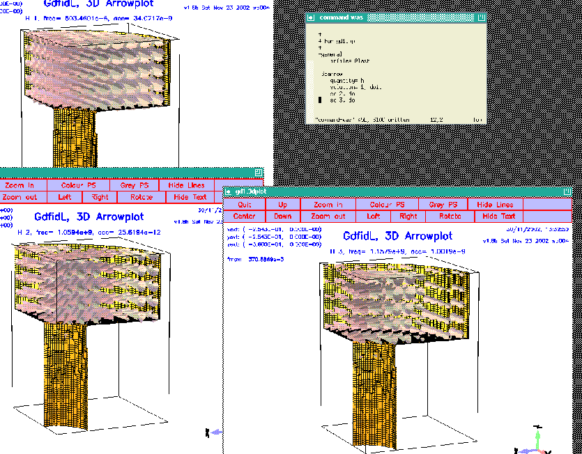
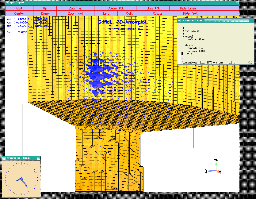
Abbreviated we may say eg.

 -3da, sy e_1, d

We can look at several plots simultaneously. We just say that we want to have another plot, and gd1.pp starts another instance of gd1.3dplot to show the plot. To have a look at the first three modes, we say eg.

 quantity= e
 solution= 1, doit
 so 2, doit
 so 3, doit

The figure 3.1 shows the resulting desktop.

**Figure 3.1:** Screenshot of the desktop. **gd1.pp** has popped up three instances of **gd1.3dplot**, showing the electric field of the first three modes.
$\begin{figure}\centerline{ \psfig{figure=FirstThreeModes.PS,width=524pt} }\end{figure}$

H-Fields

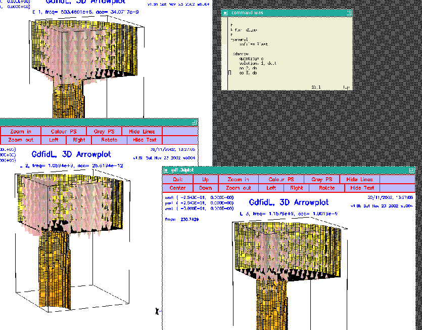When we want to look at the magnetic fields, we choose quantity= h, or we specify as symbol eg. symbol= h_1:

 -3darrow
    quantity= h
    solution= 1, doit
    solution= 2, doit
    solution= 3, doit

The figure 3.2 shows the resulting desktop.

**Figure 3.2:** Screenshot of the desktop. **gd1.pp** has popped up three instances of **gd1.3dplot**, showing the magnetic field of the first three modes.
$\begin{figure}\centerline{ \psfig{figure=FirstThree-H-Modes.PS,width=524pt} }\end{figure}$

Computing normalized shunt impedances

There are several definitions for a normalized shunt impedance floating around. We take this one:

$\begin{displaymath} R/Q = \frac{V V^*}{2 \omega W} \end{displaymath}$

(3.1)

where

is the normalized shunt impedance,
is the complex voltage that would be seen by a test charge traversing the cavity at a speed of $\beta c_0$ ,
$\omega$ is the circular frequency of the mode,
is the total stored energy in the cavity (both electric and magnetic energy).

If one evaluates the voltage seen by the test particle, one arrives at the result

$\begin{displaymath} V = \int\limits_{z=z_1}^{z=z_2} E_z(x,y,z) e^\frac{{\rm j}\omega z}{\beta c_0}\; dz \end{displaymath}$

(3.2)

for a particle that travels in positive z-direction from

We now enter the relevant sections of gd1.pp and explain how the quantities that show up in the above formula can be computed.

-lintegral: computes a line integral

To compute the complex voltage

, we enter the section -lintegral. Its menu is:

 ##############################################################################
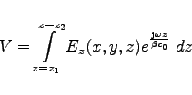
 # Flags: nomenu, prompt, message,                                            #
 ##############################################################################
 # section: -lintegral                                                        #
 ##############################################################################
 # symbol    = e_1                                                            #
 # quantity  = e                                                              #
 # solution  = 1                                                              #
 #                                                                            #
 # direction = z                                                              #
 # component = z                                                              #
 # startpoint= ( 0.0, 0.0, -1.0e+30 )                                         #
 #    (used) : ( @x0: undefined, @y0: undefined, @z0: undefined )             #
 # length    = auto                                                           #
 #    (@length) : undefined                                                   #
 # beta      = 1.0                                                            #
 # frequency = auto                     -- [auto | Real]                      #
 ##############################################################################
 # @vreal= undefined        @vimag= undefined       @vabs= undefined          #
 ##############################################################################
 # doit, ?, return, end, help                                                 #
 ##############################################################################

In order to compute our voltage, we have to specify what field shall be integrated, what component of the field shall be integrated, along which direction we want to perform the integration, and what the startpoint shall be. We specify this and perform the integration (doit):

 -lintegral
    symbol= e_1
    direction= z
    component= z
    startpoint= ( 0, 0, @zmin)
    length= auto
    doit

Upon entering "?", gd1.pp shows us the changed menu now as:

 ##############################################################################
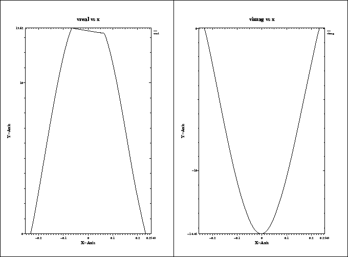
 # Flags: nomenu, prompt, message,                                            #
 ##############################################################################
 # section: -lintegral                                                        #
 ##############################################################################
 # symbol    = e_1                                                            #
 # quantity  = e                                                              #
 # solution  = 1                                                              #
 #                                                                            #
 # direction = z                                                              #
 # component = z                                                              #
 # startpoint= ( 0.0, 0.0, -360.0e-3 )                                        #
 #    (used) : ( @x0: 0.0, @y0: 0.0, @z0: -360.0e-3 )                         #
 # length    = auto                                                           #
 #    (@length) : 360.0e-3                                                    #
 # beta      = 1.0                                                            #
 # frequency = auto                     -- [auto | Real]                      #
 ##############################################################################
 # @vreal= 13.88403         @vimag= -14.67090       @vabs= 20.19905           #
 ##############################################################################
 # doit, ?, return, end, help                                                 #
 ##############################################################################

We see the startpoint that we entered is the same as the startpoint actually taken, the length of the integration path is 360 mm, and the result of the integration is: Real part is 13.88403 Volts, imaginary part is -14.67090 Volts, and the absolute value of the voltage is 20.19905 Volts. We can write these numbers down on paper, but we can also compute with them within gd1.pp. They are accessible as symbolic variables @length, @vreal, @vimag, @vabs. We will use these variables later.

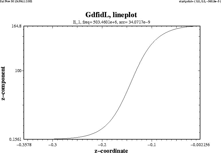
For our shunt impedance computation, we have to decide what value of the three values we have to take. From a plot of the accelerating field strength as it is shown in figure 3.3, we see that the field strength is even with respect to the plane z=0. The accelerating voltage that would be seen by a particle traversing the whole structure would therefore be twice the real part of the voltage in the half structure. In a full structure, the imaginary part of the complex voltage would vanish. We therefore have to take as four times the square of the real part @vreal.

**Figure 3.3:** component of the first mode on the axis x=y=0. Since only the part of the structure below the plane z=0 is modeled, we only have direct information about the field below z=0. Clearly, the -component is even with respect to the plane z=0.
$\begin{figure}\centerline{ \psfig{figure=ez06.PS,width=524pt} }\end{figure}$

-energy: computes stored energy in electric or magnetic field

The menu of the section -energy is:

 ##############################################################################
 # Flags: nomenu, prompt, message,                                            #
 ##############################################################################
 # section: -energy                                                           #
 ##############################################################################
 # symbol   = e_1                                                             #
 # quantity = e                                                               #
 # solution = 1                                                               #
 #                                                                            #
 #                                                                            #
 # @henergy : undefined                 (symbol: undefined, m: 1)             #
 # @eenergy : undefined                 (symbol: undefined, m: 1)             #
 ##############################################################################
 # doit, ?, return, end, help                                                 #
 ##############################################################################

We have to know both the energy in the electric field and in the magnetic field. But since the fields are resonant fields, the energies are the same for both types of fields. So it suffices to compute only the energy in the electric field:

 -energy
     quantity= e
     solution= 1
     doit

The result of the energy computation is now available in the menu, as well as the value of the symbolic variable @eenergy.

 ##############################################################################
 # Flags: nomenu, prompt, message,                                            #
 ##############################################################################
 # section: -energy                                                           #
 ##############################################################################
 # symbol   = e_1                                                             #
 # quantity = e                                                               #
 # solution = 1                                                               #
 #                                                                            #
 #                                                                            #
 # @henergy : undefined                 (symbol: undefined, m: 1)             #
 # @eenergy : 98.21061e-12              (symbol: e_1, m: 2)                   #
 ##############################################################################
 # doit, ?, return, end, help                                                 #
 ##############################################################################

Since we have modelled only the eighth part of the structure (we did use all three symmetry planes), the stored energy in the electric field of the whole structure is 8 times as high as @eenergy=98.21061e-12 Ws.

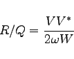
We now have all the necessary numbers to compute the normalized shunt impedance of this first mode:

The complex voltage that would be seen by a particle traversing the full cavity is two times @vreal = 13.88,
the frequency of the mode is accessible as @frequency,
the total stored energy is 8 x 2 x 98.21061e-12 Ws = 8 x 2 x @eenergy.

We can now take our pocket calculator and perform the remaining calculations, or we can use gd1.pp for it:

  echo shuntimpedance is \
   eval((2*@vreal)*(2*@vreal) / (2*@pi*@frequency * 8*2*@eenergy) ) Ohms

The full input for the postprocessor:

 -general
    infile= @last
 -energy
    symbol= e_1
    doit
 -lintegral
    component= z, direction= z
    startpoint= (0,0,@zmin)
    doit

  echo frequency is: eval(@frequency/1e6) MHz
  echo shuntimpedance is \
   eval((2*@vreal)*(2*@vreal) / (2*@pi*@frequency * 8*2*@eenergy) ) Ohms

gd1.pp tells us then:

 frequency is: 503.4601030 MHz
 shuntimpedance is  155.11998650323 Volts

Computing quality factors Q

The quality factor Q is defined as

$\begin{displaymath} Q = \frac{\omega W}{P} \end{displaymath}$

(3.3)

where

$\omega$ is the circular resonant frequency,
is the total stored energy,
is the total power loss due to currents in lossy materials.

We know already from the previous pages how to compute the stored energy. What we need now in addition is the computation of the power losses.

-wlosses: computation of wall losses with the pertubation formula

We enter the section -wlosses. Its menu is:

 ##############################################################################
 # Flags: nomenu, prompt, message,                                            #
 ##############################################################################
 # section: -wlosses                                                          #
 ##############################################################################
 # symbol    = e_1                                                            #
 # quantity  = e                                                              #
 # solution  = 1                                                              #
 # frequency = auto                     -- [auto | Real]                      #
 #                                                                            #
 #                                                                            #
 # @metalpower : undefined             (symbol: undefined)                    #
 ##############################################################################
 # doit, ?, return, end, help                                                 #
 ##############################################################################

Since the power losses are caused by currents flowing in metal, and the currents are proportional to the tangential H-field at the metallic walls, we have to enter a H-field as symbol or quantity.

 -wlosses
    quantity= h
    solution= 1
    doit

The wall losses are computed as:

$\begin{displaymath} \int \int \frac{H^2}{1 /(2 \kappa \delta)} dF \nonumber \end{displaymath}$

$\begin{displaymath} \frac{1}{\delta} = \sqrt{ \pi f \mu _0 \kappa } \nonumber \end{displaymath}$

The integral is performed over all metallic surfaces that would appear in a plot as produced by the section -3darrowplot. This implies, that wall losses are NOT computed for electric symmetry planes, since the material on the symmetry planes are not shown in -3darrowplot.

The conductivities that are used in the pertubation formula may be entered in the section -material. The result of the computation is available as the symbolic variable @metalpower.

The resulting menu (with the default conductivities of copper) is

 ##############################################################################
 # Flags: nomenu, prompt, message,                                            #
 ##############################################################################
 # section: -wlosses                                                          #
 ##############################################################################
 # symbol    = h_1                                                            #
 # quantity  = h                                                              #
 # solution  = 1                                                              #
 # frequency = auto                     -- [auto | Real]                      #
 #                                                                            #
 #                                                                            #
 # @metalpower : 16.21816e-6           (symbol: h_1)                          #
 ##############################################################################
 # doit, ?, return, end, help                                                 #
 ##############################################################################

Voltages at different paths : How to steer gd1.pp from a shell script

Our structure so far is a purely rotational symmetric one. Therefore, if the geometry would have been modelled perfectly, the shunt-impedance (for the monopole mode) at other locations (x,y)^3.1 should be exactly the same^3.2 as the shunt-impedance at (x,y)=(0,0). We now use this property of rotational symmetric structures to estimate the discretisation error we have to live with.

It suffices to compute the voltage at different paths, the stored energy of course is independent of the position (x,y). We compute the voltages at all positions (xi,0) and (0,yi) that are available in the grid. These positions of the grid planes are available in gd1.pp as the symbolic functions @x(i), @y(i), @z(i). The total number of grid planes are available as @nx, @ny, @nz. These symbols are only available after a database has been specified in -general.

So, to compute the voltages at all possible positions (xi,0) we may say:

 -lintegral
    symbol= e_1
    direction= z, component= z
    do ix= 1, @nx
       startpoint= ( @x(ix), 0, @zmin )
       doit
       echo voltage along ( @x0 , @y0 , z=z ) is @vreal @vimag @vabs
    enddo

If we do this, we get a lot of messages on the screen. In order to have a nice graphic of the dependence of the voltage on x, we better redirect the output to a file and process the result slightly. We write a small shell script:

#!/bin/sh

 #
 # feed the postprocessor with a 'here'-document,
 # 'tee' the output of the postprocessor to the file "pp.out"
 #

 (gd1.pp | tee pp.out) << EOF

    nomenu, noprompt, nomessage     # no unneccessary output
    -general, infile= @last
    -lintegral
       symbol= e_1
       direction= z, component= z
       do ix= 1, @nx
          startpoint= ( @x(ix), 0, @zmin )
          doit
          echo @x0 @vreal @vimag # <= x, vreal, vimag
       enddo
    end
EOF

 #
 # Write a PlotMtv-header to "x-voltages.mtv".
 #
 # Process the file "pp.out":
 # 'grep' the lines with the pattern "vreal"
 #
 echo \$ DATA= COLUMN  >  x-voltages.mtv
 echo x vreal  vimag   >> x-voltages.mtv

 grep vreal pp.out     >> x-voltages.mtv

 #
 # now start "mymtv2" to display the data:
 #
 mymtv2 -mult -landscape x-voltages.mtv

3.4 This shell-script can be found as "/usr/local/gd1/Tutorial-SRRC/x-voltages.x". The resulting plot is shown in figure 3.4. We see that the real part of the integrated voltage is almost constant in the range $\vert x\vert < 0.065$ m. The value of 0.065 m is the radius of the entrance of the cavity. The imaginary part is not constant, but it would be, if we would have modelled the full z-length of the geometry (it would be zero then).

**Figure 3.4:** The real part and imaginary part of the integrated voltage as a function of the position x. This plot has not been generated directly by **gd1.pp**, but has been produced by a simple shell-script.
$\begin{figure}\centerline{ \psfig{figure=x-voltages.PS,width=524pt} }\end{figure}$

Computing Wakepotentials

In order to compute wakepotentials, we have to perform a time domain computation with a line charge as excitation. The line charge travels with the velocity of light in z-direction. Since there is only one charge traveling in positive z-direction, we loose a symmetry plane. We change the borders of the computational volume to:

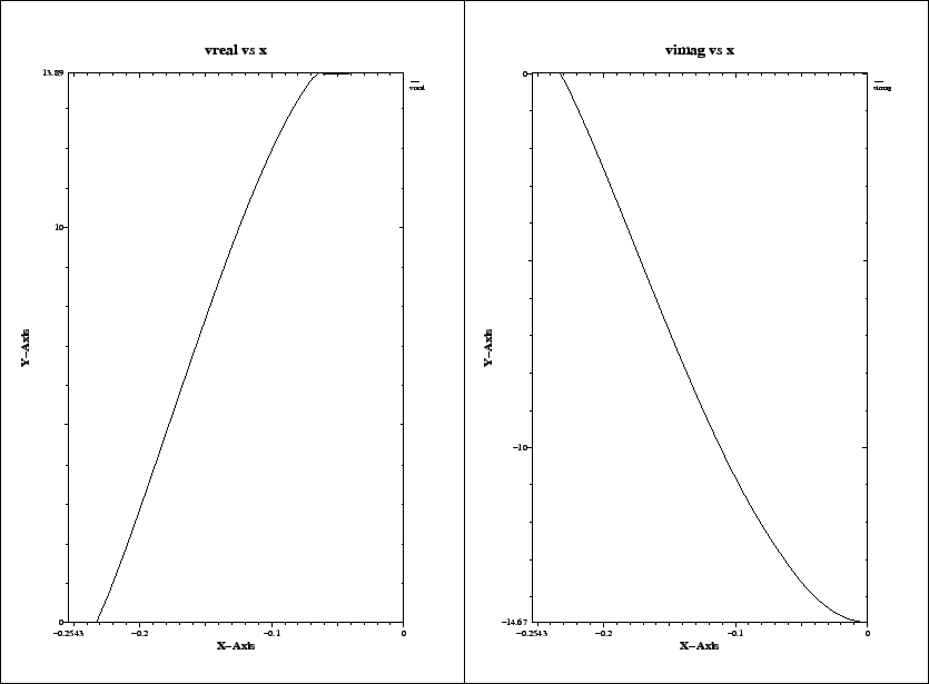 -mesh
define(STPSZE, InnerRadius/15)
     spacing= STPSZE
     pxlow= -1.1*OuterRadius
     pylow= -1.1*OuterRadius
     pzlow = -(GapLength/2+TaperLength+9e-2)
     pxhigh= 0
     pyhigh= 0
     pzhigh=  (GapLength/2+TaperLength+9e-2)

For the linecharge, we have to specify its total charge, its length, and the (x,y)-position where it shall travel. We also have to say that we do not want to compute eigenvalues, but we want to perform a time domain computation. We specify that at the lower and upper z-planes absorbing boundary conditions shall be applied. In the section -time, we specify that we want to have saved the fields at 90 equidistant times between the time that the line charge has traveled 0.1 m and it has traveled 1 m.

We edit our inputfile, such that the end of it looks as:

 -eigenvalues
    solutions= 15
    estimation= 2e9   # the estimated highest frequency
#     doit

 -fdtd
    -lcharge
        charge= 1e-12
        sigma= 4*STPSZE
        xposition= 0, yposition= 0
        shigh= 1.5
        showdata= yes

    -ports
        name= beamlow , plane= zlow, modes= 3, npml= 40, doit
        name= beamhigh, plane= zhigh, modes= 3, npml= 40, doit

    -time
        firstsaved= 0.1/@clight
        lastsaved= 1/@clight
        distancesaved= 0.1/@clight

 -fdtd
    doit

The so edited inputfile can be found as "/usr/local/gd1/Tutorial-SRRC/doris05-wake.gdf". We start the computation by feeding gd1 the inputfile:

 gd1 < doris05-wake.gdf | tee out

The computation only takes some minutes, since we compute a short range wake. When the time domain iteration starts, gd1 detects that the specified wake path is tangential to two magnetic walls. gd1 spits out:

 ## I am iterating Yee's algorithm..
 ###################
 # wake-computation:
 # (x,y)-position of the line charge:
 # specified (x,y)-position : (    0.00000000    ,     0.00000000    )
 # used      (x,y)-position : (    0.00000000    ,     0.00000000    )
 # ix, iy         :                60,                60
 # min. distances :    0.00000000      ..    0.00000000
 ############ I am checking the beam-path..
 #-- charge travels at upper x-plane.
 #-- charge travels at upper y-plane.
 #########################
 # Wake computation:
 # Since the charge travels along one or two symmetry-planes,
 # only 25 % of the charge is considered traveling through
 # the computational volume.
 # The excited fields in the subvolume will be the same as if
 # you were computing without the symmetry planes.
 # The lossfactors as computed by the post-processor will be
 # the same also.
 #########################

The end of the output of gd1 (on a reasonably fast machine) is:

 timestep=      800, simulated time=    6.2198e-9  s
 wakepotentials are known up to s=    1.1353     m
 cpu time/sec: used:    64.11, since last call:     7.41, MFLOPs/s:   88.69
 Wall clock time:    71.00     s,                         MFLOPs/s:   80.08
 timestep=      900, simulated time=    6.9973e-9  s
 wakepotentials are known up to s=    1.3672     m
 cpu time/sec: used:    71.52, since last call:     7.41, MFLOPs/s:   89.45
 Wall clock time:    79.00     s,                         MFLOPs/s:   80.98
  The highest simulation time is reached .., I am stopping
 ################################
 # cpu-seconds for FDTD :       75
 # start date           : 30/11/2002
 # end date             : 30/11/2002
 # start time           : 14:00:07
 # end time             : 14:02:14
 ## This is the normal end. Don't worry.
 ## Start the postprocessor to look at the results.
 stop FDTDLoop

Looking at Wakepotentials

We now take the advice and start gd1.pp to look at the results. We give gd1.pp the following commands:

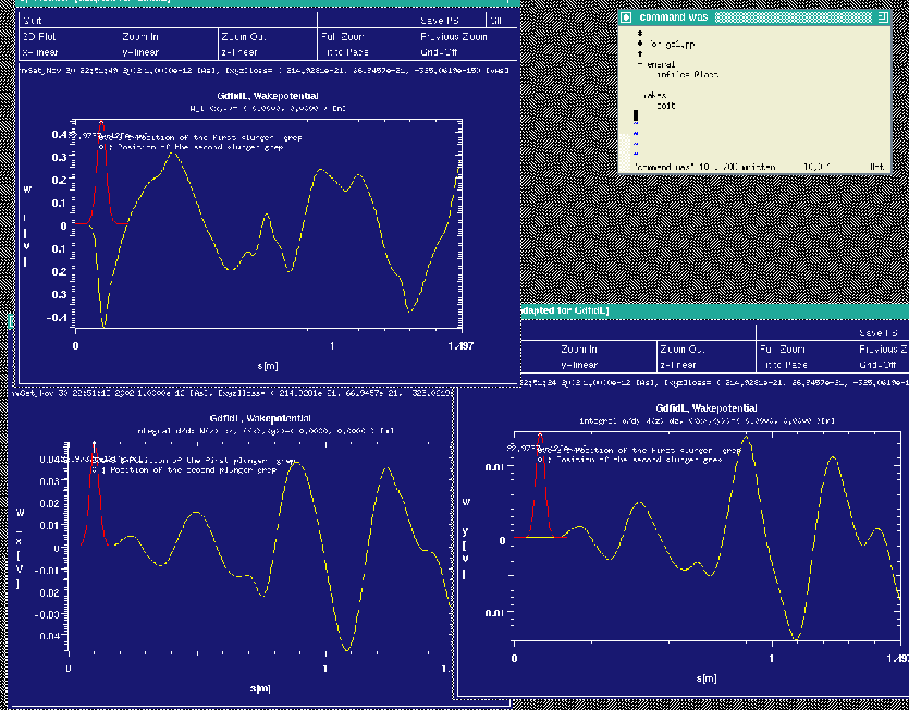
 -general
     infile= @last
 -wakes
     doit

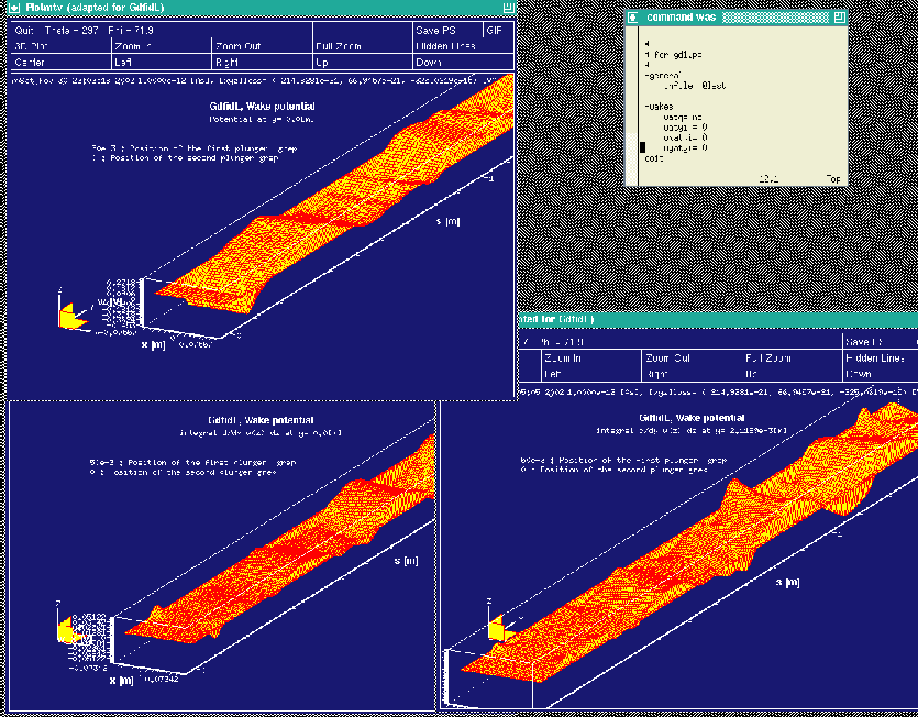
This is: We load the database of the last run, then we enter the section -wakes and start the computation of the wake-potentials with the default values. gd1.pp then computes the wakepotentials from the data that were recorded by gd1. gd1.pp starts three instances of mymtv2 to show the plots of the computed longitudinal and transverse wakepotentials. The resulting screen is shown in figure 4.1.

**Figure 4.1:** Screenshot of the desktop when the default values in -wakes are used. The three instances of **mymtv2** show the longitudinal and transverse wakepotentials at the position of the line charge, ie at the position (x,y)=(0,0). The yellow curves show the wakepotentials, the red curves show the used line-charge density. The upper left **mymtv2** shows the longitudinal wakepotential, while the lower two **mymtv2**-windows show the transverse wakepotentials.
$\begin{figure}\centerline{ \psfig{figure=wake-screen00.PS,width=524pt} }\end{figure}$

Since the structure in reality is rotational symmetric, and the charge is traveling on the axis, the longitudinal wakepotential should be independent of the (x,y) position of the test-charge. Also, the transverse wakepotentials should vanish everywhere. But since GdfidL is a 3D-code that computes in cartesian coordinates, the discretised geometry is not exactly rotational symmetric. This is the reason why the transverse wakepotentials do not vanish exactly. The computed transverse wakepotentials are 15 orders of magnitude lower than the computed longitudinal wakepotential, though.

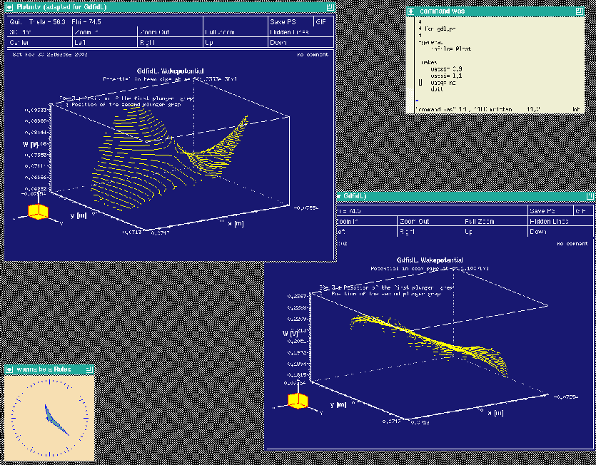
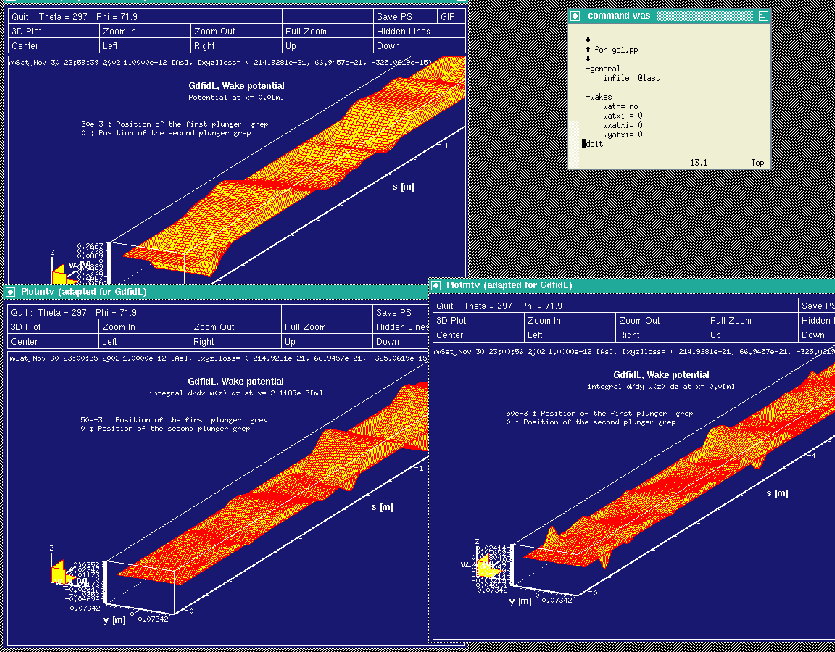
gd1.pp offers the choice to look at the longitudinal or transverse wakepotentials also as a function of (x,s) at a specified plane y=y0 or as a function of (y,s) at a specified plane x=x0.

We want to look at

the longitudinal wake in the plane x=0,
and the x-wake in the plane x=0

We enter the commands

 watxi= 0
 wxatxi= 0
 doit

The resulting screen is shown in figure 4.2.

**Figure 4.2:** Screenshot of the desktop when the plots of wakes in a plane are requested. The two instances of **mymtv2** show the longitudinal and transverse wakepotentials near the plane y=0.
$\begin{figure}\centerline{ \psfig{figure=wake-screen01.PS,width=524pt} }\end{figure}$

We see that the longitudinal wakepotential is almost everywhere independent of the position x, only near the boundary this is not the case. The transverse potential, being proportional to the transverse gradient of the longitudinal wakepotential, is therefore almost everywhere 'zero', as it should be.

Looking at Wakefields

Since we specified

    -time
        firstsaved= 0.1/@clight
        lastsaved= 1/@clight
        distancesaved= 0.1/@clight

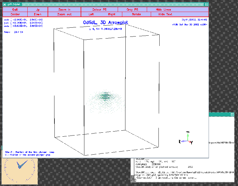
in the inputfile for gd1, gd1 did save the electric and magnetic fields at several times. We look at the fourth saved electric field:

 -3darrow
     symbol= e_4
     arrows= 40000 # default is 1000
                   # but for wakefields, better take more
     doit

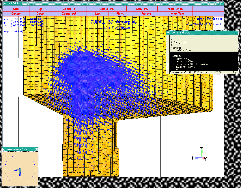
The resulting plot is shown in figure 4.3

**Figure 4.3:** The electric field as induced by a line charge traveling on the axis. The direction of the arrows indicate the direction of the field, and their size is proportional to the absolute value of the field strength.
$\begin{figure}\centerline{ \psfig{figure=wakefield00.PS,width=524pt} }\end{figure}$

Since the field near the line charge is extremely large (it is singular in reality), we see mostly field near the charge. In order to see the field away from the line charge, we specify that we want to magnify the arrows by a factor of 20, but we do not want to have any arrow larger than "2":

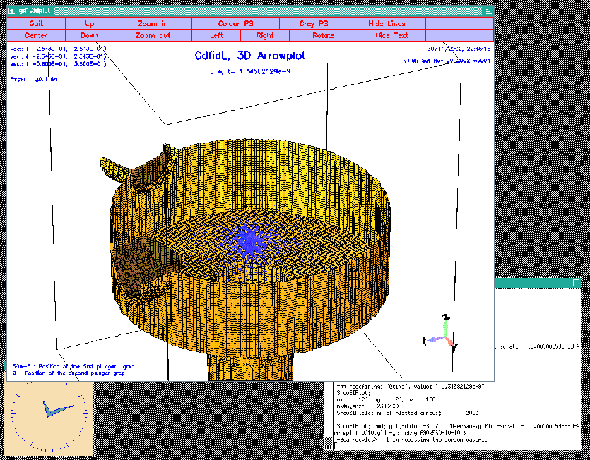
 -3darrow
     symbol= e_4
     arrows= 40000    # default is 1000 
                      # but for wakefields, better take more
     lenarrows= 20    # <- magnify
     maxlenarrows= 2  # .. but no arrow larger than "2"
     doit

The resulting plot is shown in figure 4.4

**Figure 4.4:** The electric field as induced by a line charge traveling on the axis. The direction of the arrows indicate the direction of the field. Their size now is not proportional to the field strength, since we did specify that there should be a treshold value of "maxlenarrows= 2".
$\begin{figure}\centerline{ \psfig{figure=wakefield01.PS,width=524pt} }\end{figure}$

Analysing the real 3D geometry

Modelling the geometry

The technical drawings that we have indicate that there are two tuning plungers attached. There is also a pumping hole and some device that might be the coupling loop. We ignore the pumping hole and the coupling loop now and model the two plungers.

**Figure 5.1:** The technical drawing with the plungers, pumping hole and feeding loop.
$\begin{figure}\centerline{ \psfig{figure=cavity02.PS,width=12cm,bbllx=1pt,bblly=1pt,bburx=599pt,bbury=799pt,clip=} }\end{figure}$

Modelling a Plunger

Both plungers are topologically the same. They consist of a tube where inside of the tube a circular cylinder with a rounded cap sits in.

**Figure 5.2:** Details of the technical drawing, showing the plungers.
$\begin{figure}\centerline{ \psfig{figure=cavity03.PS,width=8cm,bbllx=90pt,bblly... ...S,width=8cm,bbllx=31pt,bblly=80pt,bburx=565pt,bbury=637pt,clip=} }\end{figure}$

**Figure 5.3:** An outline of the body of revolution that shall decribe the body of a plunger.
$\begin{figure}\centerline{ \psfig{figure=plunger00.PS,width=7cm,bbllx=1pt,bblly=41pt,bburx=529pt,bbury=775pt,clip=} }\end{figure}$

A plunger is a body of revolution. gd1 can model this directly. We edit our inputfile so that it contains:

 #
 # a plunger
 #
 define(PlungerRadius0, 110e-3/2 )
 define(PlungerInnerRadius, 100e-3/2 )
 define(PlungerCurvature, 16e-3)

 -gbor
     material= 10
     originprime= (0,0,0)
     zprimedirection= (0,0,1)
     rprimedirection= (1,0,0)
     range= (0,360)

     clear
        # point= (z,r)
     point= ( 0,0 )
     point= ( 0, PlungerInnerRadius-PlungerCurvature )
        arc, radius= PlungerCurvature, size= small, type= counterclockwise
     point= ( -PlungerCurvature, PlungerInnerRadius )
     point= ( -170e-3, PlungerInnerRadius )
     point= ( -170e-3, 0 )
 show= now,
     doit

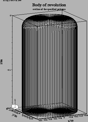
The figure 5.3 shows an outline of the body of revolution that this decribes. This plunger has its axis direction in z-direction. Our plungers shall have their axis lying in the x-y-plane, with an angle of -90+22.5 and 17 degrees. In order to have the axis of our plunger direct in the proper direction, we change the values of zprimedirection, rprimedirection. These two vectors define the local z', r' coordinate-system, in which the body of revolution is described. We edit our inputfile:

 define(PlungerAngle, (-90+22.5)*@pi/180 )
     originprime= (0,0,0)
     zprimedirection= ( -cos(PlungerAngle) ,\
                        -sin(PlungerAngle) ,\
                        0 )
     rprimedirection= ( 0, 0, 1 )

The resulting outline is shown in figure 5.4.

**Figure 5.4:** The plunger now has its axis showing in the right direction.
$\begin{figure}\centerline{ \psfig{figure=plunger01.PS,width=14cm,bbllx=1pt,bblly=7pt,bburx=778pt,bbury=575pt,clip=} }\end{figure}$

We are not done yet: The plunger is not yet at the right position. The origin of the plunger shall not be at (x,y,z)=(0,0,0), but at (x,y,z)=( $r \cos(\varphi), r \sin(\varphi), 0$ ), with $\varphi = -90+25$ degrees. We change our inputfile:

 define(PlungerRadius0, OuterRadius-50e-3 )
 define(PlungerAngle, (-90+22.5)*@pi/180 )
     originprime= ( cos(PlungerAngle)*PlungerRadius0 ,\
                    sin(PlungerAngle)*PlungerRadius0 ,\
                    0 )
     zprimedirection= ( -cos(PlungerAngle) ,\
                        -sin(PlungerAngle) ,\
                       0 )
     rprimedirection= ( 0, 0, 1 )

When we feed gd1 with this inputfile, we do not see the plunger in the plot of the material-discretisation. The reason is: The plunger is outside of the specified computational volume. Since the geometry with the plunger does no longer have all three symmetry-planes, we have to compute in a much larger volume. The only symmetry plane left is the plane z=0. So we change the specifications for the boundaries of the computational volume to:

 ###
 ### We define the borders of the computational volume,
 ### we define the default mesh-spacing,
 ### and we define the conditions at the borders:
 ###
 -mesh
     spacing= InnerRadius/15
     pxlow= -1.1*OuterRadius
     pylow= -1.1*OuterRadius
     pzlow = -(GapLength/2+TaperLength+9e-2)
     pxhigh=  1.1*OuterRadius
     pyhigh=  1.1*OuterRadius
     pzhigh= 0

     #
     # The conditions to use at the borders of the computational volume:
     #
     cxlow= electric, cxhigh= electric
     cylow= electric, cyhigh= electric
     czlow= electric, czhigh= electric

The so edited inputfile can be found as "/usr/local/gd1/Tutorial-SRRC/wPlunger00.gdf". When we feed gd1 with this inputfile (gd1

wPlunger00.gdf), we see a picture similiar as the one shown in figure 5.5

**Figure 5.5:** Screenshot of the desktop when the inputfile wPlunger00.gdf has been fed into **gd1**.
$\begin{figure}\centerline{ \psfig{figure=plunger-screen00.PS,width=524pt} % 1276/3 = 425.333333 }\end{figure}$

Using macros to model two plungers

Since we have to model two plungers, we could edit our inputfile to contain the description of the other plunger as well. But this is a good opportunity to use a macro.

Anywhere in an inputfile we can define macros. A macro is enclosed between two lines: The first line contains the keyword macro followed by the name of the macro. All lines until a line with only the keyword endmacro are considered the body of the macro. When gd1 or gd1.pp find such a macro, they read it and store the body of the macro in an internal buffer.

Example

   #
   # This defines a macro with name 'foo'
   #
   macro foo
      echo I am foo, my first argument is @arg1
      echo The total number of arguments supplied is @nargs
   endmacro

When gd1 or gd1.pp find a call of the macro, the number of the supplied arguments is assigned to the variable @nargs, and the variables @arg1, @arg2, .. are assigned the values of the supplied parameters of the call. The values of the arguments are strings. Of course it is possible to have a string eg. '1e-4' which happens to be interpreted in the right context as a real number.

Example

   #
   # this calls 'foo' with the arguments 'hi', 'there'
   #
   call foo(hi, there)

Macro calls may be nested. The body of a macro may call another macro.

Macro 'InnerPlunger'

Since the two plungers are at different angles, and their radial positions are to be changed, we parameterize our macro with arguments. We define a macro 'InnerPlunger' that expects two arguments: The first argument is the radius where the plunger shall be placed, and the second argument is the angle of the axis of the plunger:

 #
 # a plunger
 #
 macro InnerPlunger
    define(PlungerRadius0, @arg1         )  # Argument of the call
    define(PlungerAngle,   @arg2*@pi/180 )  # Argument of the call
    define(PlungerInnerRadius, 100e-3/2  )
    define(PlungerCurvature, 16e-3)

    -gbor
        material= 10
        origin= ( cos(PlungerAngle)*PlungerRadius0 ,\
                  sin(PlungerAngle)*PlungerRadius0 ,\
                 0 )
        zprimedirection= ( -cos(PlungerAngle)*PlungerRadius0 ,\
                           -sin(PlungerAngle)*PlungerRadius0 ,\
                          0 )
        rprimedirection= (0,0,1)
        range= (0,360)

        clear
           # point= (z,r)
        point= (0,0)
        point= (0, PlungerInnerRadius-PlungerCurvature )
           arc, radius= PlungerCurvature, size= small, type= counterclockwise
        point= ( -PlungerCurvature, PlungerInnerRadius )
        point= ( -170e-3, PlungerInnerRadius )
        point= ( -170e-3, 0)
        doit
 endmacro # InnerPlunger

Macro 'OuterPlunger'

Since the tubes where the plungers are in are of different radii, and they are at different angles, we must supply these parameters. For the tube where the plunger is in, we define a macro 'OuterPlunger' that expects two arguments: The first is the radius of the tube, the second one is the angle of the axis of the tube:

 macro OuterPlunger
    define(PlungerOuterRadius, @arg1 )
    define(PlungerAngle,   (@arg2)*@pi/180 )  # Argument of the call

    -gbor
        material= 0
        origin= ( cos(PlungerAngle)*OuterRadius,\
                  sin(PlungerAngle)*OuterRadius,\
                  0 )
        zprimedirection= ( -cos(PlungerAngle),\
                           -sin(PlungerAngle),\
                          0 )
        rprimedirection= (0,0,1)
        range= (0,360)

        clear
           # point= (z,r)
        point= (  50e-3, 0 )
        point= (  50e-3, PlungerOuterRadius )
        point= (  50e-3, PlungerOuterRadius )
        point= ( -235.39e-3, PlungerOuterRadius )
        point= ( -235.39e-3, 50e-3)
        point= ( -235.39e-3, 0)
        doit
 endmacro # OuterPlunger

We now model each of our two plungers with two calls:

 #
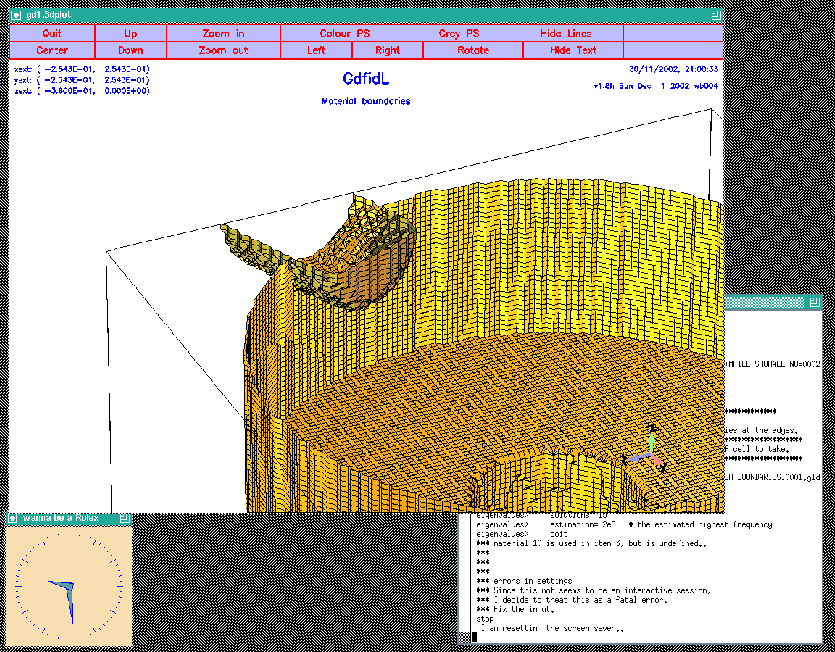
 # Model the tube and the plunger at phi=17 degrees:
 #
 call OuterPlunger( (130.75e-3/2)      , 17 )
 call InnerPlunger( (OuterRadius-50e-3), 17 )

 #
 # model the tube and the plunger at phi=-90+22.5 degrees:
 #
 call OuterPlunger( (110e-3/2)         , (-90+22.5) )
 call InnerPlunger( (OuterRadius-50e-3), (-90+22.5) )

The so edited inputfile can be found as /usr/local/gd1/Tutorial-SRRC/wPlunger01.gdf. When we feed gd1 with this inputfile, we get a screen as shown in figure 5.6.

**Figure 5.6:** Screenshot of the desktop when the inputfile wPlunger01.gdf has been fed into **gd1**. Shown is a zoom of the interesting region near the plungers.
$\begin{figure}\centerline{ \psfig{figure=plunger-screen01.PS,width=524pt} % 1276/3 = 425.333333 }\end{figure}$

Defining Material properties

gd1 does find an error in our inputfile. It complains:

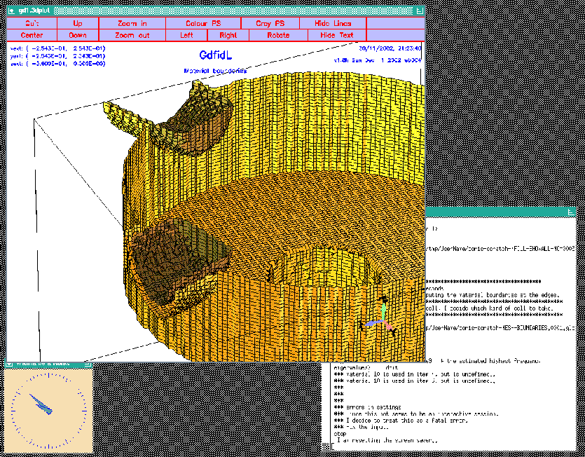 eigenvalues>     solutions= 15
 eigenvalues>     estimation= 2e9   # the estimated highest frequency
 eigenvalues>     doit
 *** material 10 is used in item 4, but is undefined..
 *** material 10 is used in item 6, but is undefined..
 *** errors in settings
 *** Since this not seems to be an interactive session,
 *** I decide to treat this as a fatal error.
 *** Fix the input.
 stop

gd1 complains that we used a material index of '10' to model our plungers. The properties of this material '10' have not yet been defined. We doit by editing our inputfile, such that before the eigenvalue computation starts, we have:

 -material           # enter the section "-material"
     material= 10    # the properties of material "10" shall be changed.
     type= electric  # shall be treated as perfect electric conducting
                     # for the field computation

We did use the materials '0' and '1' as well. We did not define the properties of them, but the default values of these materials are what we want (material '0' is vacuum, material '1' is copper, and material '2' is perfect magnetic conducting).

Computing Eigenvalues

When we feed the so edited inputfile to gd1 (gd1

wPlunger02.gdf), gd1 gives as final table (on a reasonably fast machine):

 boundary conditions:
 xboundary= electric, electric
 yboundary= electric, electric
 zboundary= electric, electric
 
  --------------------
 
    i   freq(i)       acc(i)         cont(i)
    1  436.4010e+6   1.0044982017  1.0000000000       # "grep" for me
    2  508.3705e+6   0.0014197280  0.0014201239       # "grep" for me
    3  782.2763e+6   0.0000381458  0.0000535041       # "grep" for me
    4  785.5885e+6   0.0002404450  0.0003882672       # "grep" for me
    5    1.0476e+9   0.0000318869  0.0000629098       # "grep" for me
    6    1.0620e+9   0.0002907024  0.0049598724       # "grep" for me
    7    1.0930e+9   0.0002534295  0.0044621769       # "grep" for me
    8    1.0985e+9   0.0001211415  0.0014816978       # "grep" for me
    9    1.1436e+9   0.0003028035  0.0023958708       # "grep" for me
   10    1.2149e+9   0.0040771062  0.0350091443       # "grep" for me
   11    1.2437e+9   0.0074278316  0.1613287149       # "grep" for me
   12    1.2652e+9   0.0671920760  1.0000000000       # "grep" for me
   13    1.2845e+9   0.0265391147  0.5529007301       # "grep" for me
   14    1.3151e+9   0.0376288530  0.3142827624       # "grep" for me
   15    1.3935e+9   0.0930865808  0.8046319226       # "grep" for me
 ################################
 # cpu-seconds for eigenvalues :      472
 # start date                  : 30/11/2002
 # end date                    : 30/11/2002
 # start time                  : 21:41:36
 # end time                    : 21:50:45
 # The computation of the eigenvalues has finished normally..
 # Start the postprocessor to look at the results.
 stop .. normal end ..

The first mode is garbage, as can be seen from its accuracy. But also the other modes are not very good. The reason is: Since we have only a single symmetry plane left (z=0), we have to compute in a volume that is four times as large as the volume before. In such a large volume, there are much more modes than 15 in the frequency range from 0 to estimation (we specified an estimation of 2GHz). We could say that we want to have more solutions, but that would drastically increases our memory consumption. Since we are using already about 200 MBytes (our grid contains 1.2 million gridcells), we do not want to do this. We could try to compute with the single precision version of gd1, single.gd1, then we could compute 30 modes in 200 MByte. Instead we adjust our estimation to 1.2 GHz. The end of our inputfile now is:

 -eigenvalues
    solutions= 15
    estimation= 1.2e9   # the estimated highest frequency
    doit

and the final table of a run (gd1

wPlunger03.gdf) is

 boundary conditions:
 xboundary= electric, electric
 yboundary= electric, electric
 zboundary= electric, electric
 
  --------------------
 
  The first 2 solutions seem to be static and are not saved.
    i   freq(i)       acc(i)         cont(i)
    1  508.3705e+6   0.0000027120  0.0000022258       # "grep" for me
    2  782.2764e+6   0.0000000527  0.0000000740       # "grep" for me
    3  785.5885e+6   0.0000000113  0.0000000182       # "grep" for me
    4    1.0476e+9   0.0000000021  0.0000000042       # "grep" for me
    5    1.0620e+9   0.0000000009  0.0000000155       # "grep" for me
    6    1.0930e+9   0.0000000245  0.0000004322       # "grep" for me
    7    1.0985e+9   0.0000000053  0.0000000651       # "grep" for me
    8    1.1436e+9   0.0000000643  0.0000005090       # "grep" for me
    9    1.2149e+9   0.0000675156  0.0005797832       # "grep" for me
   10    1.2434e+9   0.0000015519  0.0000339391       # "grep" for me
   11    1.2587e+9   0.0000055368  0.0001618450       # "grep" for me
   12    1.2801e+9   0.0006670306  0.0200800431       # "grep" for me
   13    1.2994e+9   0.0015633650  0.0522703164       # "grep" for me
 ################################
 # cpu-seconds for eigenvalues :      747
 # start date                  : 30/11/2002
 # end date                    : 30/11/2002
 # start time                  : 21:52:37
 # end time                    : 22:06:21
 # The computation of the eigenvalues has finished normally..
 # Start the postprocessor to look at the results.
 stop .. normal end ..

The garbage mode has disappeared, and the accuracies the modes are very good.

Using gd1.pp to analyse the results

Transverse Kickfactors

Since our structure is no longer rotational symmetric, the shunt-impedance of the monopole-mode is no longer independent of the position of the testcharge. Since a real charge cloud has a finite extension in the x-y plane, the charges at different (x,y) positions will experience a different accelerating voltage. This gives rise to an energy spread. We can again use the shell-script of page

to compute the variation of the accelerating voltage as a function of the x-position. For convenience, the shell script '/usr/local/gd1/Tutorial-SRRC/x-voltages.x' is shown here again:

#!/bin/sh

 #
 # feed the postprocessor with a 'here'-document,
 # 'tee' the output of the postprocessor to the file "pp.out"
 #

 (gd1.pp | tee pp.out) << EOF

    nomenu, noprompt, nomessage     # no unneccessary output
    -general, infile= @last
    -lintegral
       symbol= e_1
       direction= z, component= z
       do ix= 1, @nx
          startpoint= ( @x(ix), 0, @zmin )
          doit
          echo @x0 @vreal @vimag # <= x, vreal, vimag
       enddo
    end
EOF

 #
 # Write a PlotMtv-header to "x-voltages.mtv".
 #
 # Process the file "pp.out":
 # 'grep' the lines with the pattern "vreal"
 #
 echo \$ DATA= COLUMN  >  x-voltages.mtv
 echo x vreal  vimag   >> x-voltages.mtv

 grep vreal pp.out     >> x-voltages.mtv

 #
 # now start "mymtv2" to display the data:
 #
 mymtv2 -mult -landscape x-voltages.mtv

The resulting plot is shown in figure 7.1.

**Figure 7.1:** A plot of the real part and imaginary part of the accelerating voltage of the monopole mode in the cavity with plungers. Only the real part would be nonzero, if the symmetry plane at z=0 would not have been used. One can clearly see that the accelerating voltage no longer is independent of the x-position.
$\begin{figure}\centerline{ \psfig{figure=x-voltages-with-plungers.00.PS,width=15cm} }\end{figure}$

There will of course be a variation of the voltage on the y-position as well. One could analyse this with a similiar shell script.

Frequencies as a function of the position of a plunger

The plungers will not have a fixed radial position, but they will be used for tuning the cavity. To analyse the effect of the position of the plungers on some electric property of the cavity, we can compute many different plunger positions and analyse the result. To compute many different plunger positions, one could edit the inputfile for each positions and compute. This would tediuos. There must be a better way.

Steering gd1 or gd1.pp from a shell script

We can steer gd1 or gd1.pp by adding an option -Dname=value when starting the program. gd1 then defines a symbolic variable with name name to have the value value. The effect is therefore the same as if in the very first line of its input, the line sdefine(name, value) would occur. We write a small shell script that starts gd1 three times with three different values for the option.

#!/bin/sh

 for POS1 in 0e-3 25e-3 50e-3
 do
     gd1 -Dposition1=$POS1 -Dposition2=0 \
        < /usr/local/gd1/Tutorial-SRRC/wPlunger04.gdf | tee out.pos1=$POS1
 done

This shell-script can be found as '/usr/local/gd1/Tutorial-SRRC/many-pos1.x'. The inputfile 'wPlunger04.gdf' now calls the macros as follows:

 #
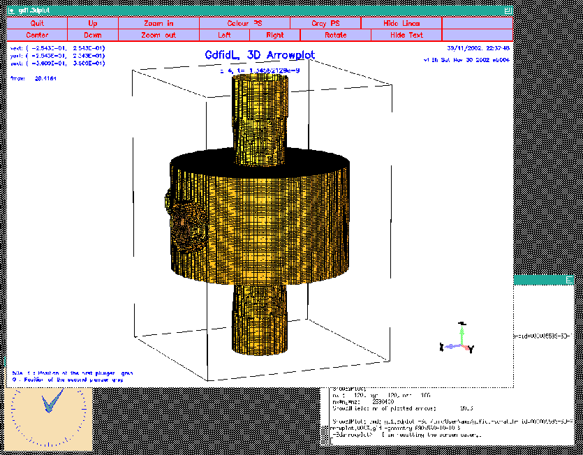
 # Model the tube and the plunger at phi=17 degrees:
 #
 call OuterPlunger( (130.75e-3/2)          , 17 )
 call InnerPlunger( (OuterRadius-position1), 17 )

 #
 # model the tube and the plunger at phi=-90+22.5 degrees:
 #
 call OuterPlunger( (110e-3/2)             , (-90+22.5) )
 call InnerPlunger( (OuterRadius-position2), (-90+22.5) )

The actual positions are output as annotations by specifying in the section -general:

 -general
    text()= position1 : Position of the first plunger  grep
    text()= position2 : Position of the second plunger grep

When gd1 reads this, it will substitute the 'position1' with the value that was supplied to it via its commandline option -Dposition1=$POS1, the corresponding happens to the string 'position2'. The strings 'grep' are supplied so that the outputfiles out.pos1=$POS1 can be 'grep'ed for the string 'grep'. The full inputfile can be found as /usr/local/gd1/Tutorial-SRRC/wPlunger04.gdf'.

When we run our shell script, we get three files

   out.pos1=0e-3, out.pos1=25e-3, out.pos1=50e-3

where the computed frequencies can be found in. The relevant lines can be easily extracted with the UNIX-command 'grep'. To show all lines in the files out.pos* that contain the string 'grep', you say

 grep grep out.pos*

The result is:

out.pos1=0e-3: general>     text()= 0e-3 : Position of the first plunger  grep
out.pos1=0e-3: general>     text()= 0 : Position of the second plunger grep
 Position of the first plunger: 0e-3  grep
 Position of the second plunger: 0 grep
out.pos1=0e-3:    1   52.7470e+06  1.0090174050  0.3438316719       # "grep" for me
out.pos1=0e-3:    2  502.5682e+06  0.0000031370  0.0000025505       # "grep" for me
out.pos1=0e-3:    3  778.1484e+06  0.0000000660  0.0000000914       # "grep" for me
out.pos1=0e-3:    4  779.3503e+06  0.0000000163  0.0000000249       # "grep" for me
out.pos1=0e-3:    5    1.0554e+09  0.0000000001  0.0000000002       # "grep" for me
out.pos1=0e-3:    6    1.0591e+09  0.0000000003  0.0000000045       # "grep" for me
out.pos1=0e-3:    7    1.0971e+09  0.0000000012  0.0000000173       # "grep" for me
out.pos1=0e-3:    8    1.0973e+09  0.0000000045  0.0000000428       # "grep" for me
out.pos1=0e-3:    9    1.1560e+09  0.0000000521  0.0000005213       # "grep" for me
out.pos1=0e-3:   10    1.1976e+09  0.0000001260  0.0000013792       # "grep" for me
out.pos1=0e-3:   11    1.2515e+09  0.0004255555  0.0049426207       # "grep" for me
out.pos1=0e-3:   12    1.2656e+09  0.0016319888  0.0731105041       # "grep" for me
out.pos1=0e-3:   13    1.2668e+09  0.0025985547  1.0000000000       # "grep" for me
out.pos1=25e-3: general>     text()= 25e-3 : Position of the first plunger  grep
out.pos1=25e-3: general>     text()= 0 : Position of the second plunger grep
out.pos1=25e-3: 25e-3 : Position of the first plunger  grep
out.pos1=25e-3: 0 : Position of the second plunger grep
out.pos1=25e-3:    1  503.7682e+06  0.0000024488  0.0000019899       # "grep" for me
out.pos1=25e-3:    2  779.4209e+06  0.0000000124  0.0000000171       # "grep" for me
out.pos1=25e-3:    3  781.0514e+06  0.0000000431  0.0000000660       # "grep" for me
out.pos1=25e-3:    4    1.0575e+09  0.0000000027  0.0000000051       # "grep" for me
out.pos1=25e-3:    5    1.0595e+09  0.0000000002  0.0000000024       # "grep" for me
out.pos1=25e-3:    6    1.0968e+09  0.0000000062  0.0000000913       # "grep" for me
out.pos1=25e-3:    7    1.0975e+09  0.0000000018  0.0000000174       # "grep" for me
out.pos1=25e-3:    8    1.1555e+09  0.0000000372  0.0000003780       # "grep" for me
out.pos1=25e-3:    9    1.2018e+09  0.0000002208  0.0000025548       # "grep" for me
out.pos1=25e-3:   10    1.2529e+09  0.0007020442  0.0086314595       # "grep" for me
out.pos1=25e-3:   11    1.2675e+09  0.0009580488  0.0414770393       # "grep" for me
out.pos1=25e-3:   12    1.2746e+09  0.0020655866  0.1865897939       # "grep" for me
out.pos1=50e-3: general>     text()= 50e-3 : Position of the first plunger  grep
out.pos1=50e-3: general>     text()= 0 : Position of the second plunger grep
out.pos1=50e-3: 50e-3 : Position of the first plunger  grep
out.pos1=50e-3: 0 : Position of the second plunger grep
out.pos1=50e-3:    1   99.6144e+06  0.9656790469  0.3479304400       # "grep" for me
out.pos1=50e-3:    2  505.2467e+06  0.0000031189  0.0000025741       # "grep" for me
out.pos1=50e-3:    3  779.6769e+06  0.0000000046  0.0000000065       # "grep" for me
out.pos1=50e-3:    4  781.9646e+06  0.0000000537  0.0000000853       # "grep" for me
out.pos1=50e-3:    5    1.0479e+09  0.0000000086  0.0000000166       # "grep" for me
out.pos1=50e-3:    6    1.0605e+09  0.0000000016  0.0000000236       # "grep" for me
out.pos1=50e-3:    7    1.0955e+09  0.0000000193  0.0000003011       # "grep" for me
out.pos1=50e-3:    8    1.0983e+09  0.0000000036  0.0000000400       # "grep" for me
out.pos1=50e-3:    9    1.1477e+09  0.0000000200  0.0000001945       # "grep" for me
out.pos1=50e-3:   10    1.2055e+09  0.0000001903  0.0000020180       # "grep" for me
out.pos1=50e-3:   11    1.2473e+09  0.0031135695  0.0463915760       # "grep" for me
out.pos1=50e-3:   12    1.2570e+09  0.0168888927  0.6785522929       # "grep" for me
out.pos1=50e-3:   13    1.2726e+09  0.0118906521  0.4821503838       # "grep" for me

This usage of gd1 is the reason, why gd1 writes the string

   "grep" for me

in the table of the frequencies.

Computing Wakepotentials

As with the cavity without plungers, when we want to compute wakepotentials, we cannot use the symmetry plane of the geometry at z=0, since the excitation with the line-charge is not symmetric. We change the borders of the computational volume to:

 ###
 ### We define the borders of the computational volume,
 ### we define the default mesh-spacing,
 ### and we define the conditions at the borders:
 ###
 -mesh
     spacing= InnerRadius/15
     pxlow= -1.1*OuterRadius
     pylow= -1.1*OuterRadius
     pzlow = -(GapLength/2+TaperLength+9e-2)
     pxhigh=  1.1*OuterRadius
     pyhigh=  1.1*OuterRadius
     pzhigh=  (GapLength/2+TaperLength+9e-2)

     #
     # The conditions to use at the borders of the computational volume:
     #
     cxlow= electric, cxhigh= electric
     cylow= electric, cyhigh= electric
     czlow= electric, czhigh= electric

For the linecharge, we have to specify its total charge, its length, and the (x,y)-position where it shall travel. We also have to say that we do not want to compute eigenvalues, but we want to perform a time domain computation. We specify that at the lower and upper z-planes absorbing boundary conditions shall be applied. In the section -time, we specify that we want to have saved the fields at 10 equidistant times between the time that the line charge has traveled 0.1 m and it has traveled 1 m.

We edit our inputfile, such that the end of it looks as:

 -eigenvalues
    solutions= 15
    estimation= 2e9   # the estimated highest frequency
#     doit

 -fdtd
    -lcharge
        charge= 1e-12
        sigma= 4*STPSZE
        xposition= 0, yposition= 0
        shigh= 1.5
        showdata= yes

    -ports
        name= beamlow , plane= zlow, modes= 3, npml= 40, doit
        name= beamhigh, plane= zhigh, modes= 3, npml= 40, doit

    -time
        firstsaved= 0.1/@clight
        lastsaved= 1/@clight
        distancesaved= 0.1/@clight

 -fdtd
    doit

The so edited inputfile can be found as /usr/local/gd1/Tutorial-SRRC/wPlunger-wake.gdf. When we feed gd1 with the edited inputfile,

 gd1 < wPlunger-wake.gdf

gd1 stops and complains

 # was: " call InnerPlunger( (OuterRadius-position1), 17 )"
 gbor> 
 gbor>   *** rnum: Bad Constant: starts here: "position1) "
  evaluate me(:lenEvaluate): "(231.15e-3-position1) "
 *** Status: "Bad factor :"p""
 *** : "(231.15e-3-position1) "
                       |
 *** Since this not seems to be an interactive session,
 *** I decide to treat this as a fatal error.
 *** Fix the input.
 stop

We did not specify what the value of the symbols position1 and position2 shall be. We do this by defining them on the commandline of gd1:

 gd1 -Dposition1=50e-3 -Dposition2=0 < wPlunger-wake.gdf

Now the computation runs. After some minutes, the last words of gd1 are:

 timestep=      900, simulated time=    6.9214e-9  s
 wakepotentials are known up to s=    1.3455     m
 cpu time/sec: used:   300.13, since last call:    31.23, MFLOPs/s:   82.67
 Wall clock time:   305.99     s,                         MFLOPs/s:   81.09
  The highest simulation time is reached .., I am stopping
 ################################
 # cpu-seconds for FDTD :      320
 # start date           : 30/11/2002
 # end date             : 30/11/2002
 # start time           : 22:25:31
 # end time             : 22:33:22
 ## This is the normal end. Don't worry.
 ## Start the postprocessor to look at the results.
 stop FDTDLoop

Analysing the results with gd1.pp

Looking at the wakefields with gd1.pp

We start gd1.pp and issue the commands:

 -general
      infile= @last
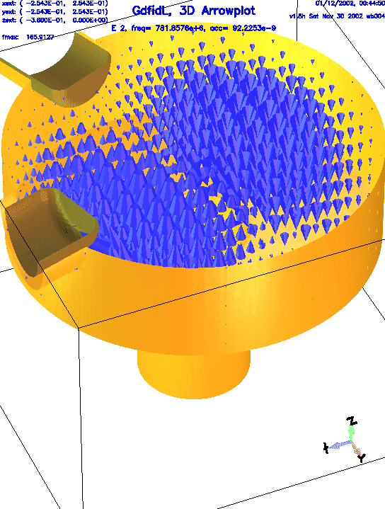
 -3darrow
     symbol= e_4
     arrows= 40000
   doit

The resulting screen is shown in figure 10.1.

**Figure 10.1:** Screenshot of the desktop showing the matrialdistribution and the wakefield at some time. We cannot see the wakefield, since the material boundaries hide the field.
$\begin{figure}\centerline{ \psfig{figure=3d-wakefield00.PS,width=524pt} }\end{figure}$

We only see the material approximation. The field is plotted inside, but we cannot see it, since the plotted material boundaries hide the field. We have several possibilities to look at the field: There is an option in this section -3darrowplot. With this option we can switch on or off the plotting of the material boundaries: materials= yes|no. The default value is materials= yes. We select

 materials= no
 doit

Now we see the field, but no material anywhere. The resulting plot is shown in figure 10.2.

**Figure 10.2:** Screenshot of the desktop when we switched off the plotting of the material-boundaries.
$\begin{figure}\centerline{ \psfig{figure=3d-wakefield01.PS,width=524pt} }\end{figure}$

We have another option to look inside the geometry. We can select that we only want to see the field and the material boundaries that are lying within some bounding box. We switch on the plotting of the materials again and specify that we do not want to see anything above z=0:

 materials= yes
 bbzhigh= 0      # don't plot anything above z=0

The resulting plot is shown in figure 10.3.

**Figure 10.3:** Screenshot of the desktop when we switched on the plotting of the material-boundaries, but selected bbzhigh=0.
$\begin{figure}\centerline{ \psfig{figure=3d-wakefield02.PS,width=524pt} }\end{figure}$

Looking at the wakepotentials

We enter the section -wakes. When we are solely interested in the longitudinal and transverse wakepotentials at the position of the line-charge, we do not have to specify any special option, the default values are good for that. The default is to compute and plot the longitudinal and transverse wakepotentials at the position of the exciting charge. We say

 -wakes
     doit

The resulting plots are shown in figure 10.4.

**Figure 10.4:** Screenshot of the desktop when we just said 'doit' in the section '-wakes'. **gd1.pp** has popped up three instances of **mymtv2** that show the longitudinal and transverse wakepotentials at the (x,y) position of the line-charge. The yellow curves are the wakepotentials, and the red curve is the charge density of the line-charge.
$\begin{figure}\centerline{ \psfig{figure=3d-wakepotentials00.PS,width=524pt} }\end{figure}$

We look at the longitudinal wakepotential as a function of (x,y) at the s-positions s=0.9m and s=1.1m by specifying

 watsi= 0.9
 watsi= 1.1
 watq= no
 doit

the watq= no instructs gd1.pp that we do not want to see again the wakepotentials at the position of the linecharge. We did specify watsi= ?? twice, this means, that we want to see the wakepotential at both s-coordinates. The resulting plots are shown in figure 10.5.

**Figure 10.5:** Screenshot of the desktop showing the longitudinal wakepotential in the cross section of the beam-pipe where a beam can travel.
$\begin{figure}\centerline{ \psfig{figure=3d-wakepotentials01.PS,width=524pt} }\end{figure}$

Wakepotentials in the plane x=0 and y=0

We can look at the wakepotentials in any plane x=x0, y=y0. When we want to look at the wakepotentials in the planes x=0 and y=0, we specify

 watxi = 0
 wxatxi= 0
 wyatxi= 0

 watyi = 0
 wxatyi= 0
 wyatyi= 0

 doit

The resulting plots are shown in the figures 10.6 and 10.7

**Figure 10.6:** Screenshot of the desktop showing the longitudinal and transverse wakepotential near the plane x=0.
$\begin{figure}\centerline{ \psfig{figure=3d-wakepotentials02.PS,width=524pt} }\end{figure}$

**Figure 10.7:** Screenshot of the desktop showing the longitudinal and transverse wakepotential near the plane y=0.
$\begin{figure}\centerline{ \psfig{figure=3d-wakepotentials03.PS,width=524pt} }\end{figure}$

This is the end of this tutorial.

Footnotes

... drawings ¹: from Mr. Ping J. Chou of the SRRC of Taiwan
... (x,y)^3.1: The locations (x,y) where the shunt impedance has to be the same are the locations where a beam can travel.
... same ^3.2: That the shunt-impedance for the monopole mode has to be constant follows from the Panofsky-Wenzel theorem.