Up: Examples Previous: Scattering Parameters Contents

Computing Brillouin-diagrams

Brillouin diagrams are plots of resonant frequencies as a function of the phase in periodic structures. GdfidL allows computation with specified phase shifts in x- y- and z-direction simultaneously. So we can compute Brillouin diagrams in 3D periodic structures, where the plane normals of the planes of periodicity are in x- y- and z-direction simultaneously.

The following inputfile defines an elemental cell of such a periodic structure.

 # /usr/local/gd1/examples-from-the-manual/brillo.gdf

 #
 # Assign a value to "PHASE", if it is not yet defined
 # via  "gd1 -DPHASE=XX"
 #
 if (! defined(PHASE) ) then
    define(PHASE, 45)
 endif

 #
 # What part of the Brillouin-diagram do we want to compute?
 #
 #
 # part==1 : from Gamma to H : 0<kx<pi/d, ky=0,      kz=0
 # part==2 : from H to N     : kx=pi/d,   0<ky<pi/d, kz=0
 # part==3 : from N to P     : kx=pi/d,   ky=pi/d,   0<kz<pi/d
 # part==4 : from P to Gamma : 0 < (kx=ky=kz) < pi/d
 #

 #
 # get the value of PART by inclusion of a file:
 # the content of the file is simply
 #    "define(PART, 1)"
 # or "define(PART, 2)"
 # or "define(PART, 3)"
 # or "define(PART, 4)"
 include(this-part-of-brillo)

 if ( PART == 1 ) then
    define(XPHASE, PHASE)
    define(YPHASE, 000)
    define(ZPHASE, 000)
 endif

 if ( PART == 2 ) then
    define(XPHASE, 180)
    define(YPHASE, PHASE)
    define(ZPHASE, 000)
 endif

 if ( PART == 3 ) then
    define(XPHASE, 180)
    define(YPHASE, 180)
    define(ZPHASE, PHASE)
 endif

 if ( PART == 4 ) then
    define(XPHASE, PHASE)
    define(YPHASE, PHASE)
    define(ZPHASE, PHASE)
 endif

 define(INF, 10000.0 *@clight)
 define(MAG, 2) define(EL, 1)

 ##
 ## Geometry definitions
 ##
 define(LATTICE_D, @clight/2 )
 define(RADIUS, LATTICE_D * 0.375 )

 #
 # default mesh spacing
 #
 define(STPSZE, RADIUS/10 )

 ##############
 ##############
 ##############
 ##############
 ##############
 -general
    outfile= /tmp/UserName/outfile
    scratchbase= /tmp/UserName/delete-me-

    text()= lattice constant d= LATTICE_D
    text()= radius of the spheres= RADIUS
    text()= r/d = eval(RADIUS/LATTICE_D)
    text()= 2r/d = eval(2*RADIUS/LATTICE_D)
    text()= stpsze= STPSZE
    text()= xphase: XPHASE
    text()= yphase: YPHASE
    text()= zphase: ZPHASE

 -mesh
    spacing= STPSZE
    graded= yes, dmaxgraded= 10*STPSZE
    qfgraded= 1.3
    perfectmesh= yes

    pxlow= -0.5*LATTICE_D, pxhigh= 0.5*LATTICE_D
    pylow= -0.5*LATTICE_D, pyhigh= 0.5*LATTICE_D
    pzlow= -0.5*LATTICE_D, pzhigh= 0.5*LATTICE_D

    xperiodic= yes, xphase= XPHASE
    yperiodic= yes, yphase= YPHASE
    zperiodic= yes, zphase= ZPHASE

    do ii= -1, 1, 1
       xfixed( 2, ii*LATTICE_D-RADIUS, ii*LATTICE_D+RADIUS )
       xfixed( 2, (ii-0.1)*LATTICE_D, (ii+0.1)*LATTICE_D )

       yfixed( 2, ii*LATTICE_D-RADIUS, ii*LATTICE_D+RADIUS )
       yfixed( 2, (ii-0.1)*LATTICE_D, (ii+0.1)*LATTICE_D )

       zfixed( 2, ii*LATTICE_D-RADIUS, ii*LATTICE_D+RADIUS )
       zfixed( 2, (ii-0.1)*LATTICE_D, (ii+0.1)*LATTICE_D )
    enddo

 ##############

 -brick
    #
    # Fill the universe with vacuum
    #
    material= 0
       volume= (-INF,INF, -INF,INF, -INF,INF)
    doit


 define(M3, 1)
 #
 # define square lattice
 # Only a part of these spheres end up being within
 # computational volume
 #
 do iz= 0, 1, 1
    do ix= 0, 1, 1
       do iy= 0, 1, 1
          #
          # a sphere with center at
          # ( ix*LATTICE_D, iy*LATTICE_D, iz*LATTICE_D )
          #
          -gbor
             material= M3
                origin= ( ix*LATTICE_D, \
                          iy*LATTICE_D, \
                          iz*LATTICE_D )
                rprimedirection= ( 1, 0, 0 )
                zprimedirection= ( 0, 0, 1 )
                range= ( 0, 360 )

                clear
                point= ( -RADIUS, 0 )
                   arc, radius= RADIUS, type= clockwise, size= small
                point= ( RADIUS, 0)
             doit
       enddo
    enddo
 enddo

 #
 # the connecting rods in x-direction
 #
 do iz= 0, 1, 1
    do iy= 0, 1, 1
       -gccylinder
          material= M3
             radius= 0.1*LATTICE_D
             length= INF
             origin= ( -INF/2, \
                       iy*LATTICE_D, \
                       iz*LATTICE_D )
             direction= ( 1, 0, 0 )
          doit
    enddo
 enddo

 #
 # the connecting rods in y-direction
 #
 do iz= 0, 1, 1
    do ix= 0, 1, 1
       -gccylinder
          material= M3
             radius= 0.1*LATTICE_D
             length= INF
             origin= ( ix*LATTICE_D, \
                       -INF/2, \
                       iz*LATTICE_D )
             direction= ( 0, 1, 0 )
          doit
    enddo
 enddo

 #
 # the connecting rods in z-direction
 #
 do ix= 0, 1, 1
    do iy= 0, 1, 1
       -gccylinder
          material= M3
             radius= 0.1*LATTICE_D
             length= INF
             origin= ( ix*LATTICE_D, \
                       iy*LATTICE_D, \
                       -INF/2 )
             direction= ( 0, 0, 1 )
          doit
    enddo
 enddo

 #
 # definition of the material properties
 #
 -material
    material= M3, type= electric


 #
 # what does the materialdistribution look like?
 #
 -volumeplot
##    doit

 #################
 #
 # computation of the eigenvalues
 #
 -eigenvalues
    solutions= 20
    estimation= 2.8
    pfac2= 1e-2
    passes= 2

    doit

 end

In order to compute the four parts of the Brillouin diagram, we use a shell-script. This shell script starts a program four times. That program starts gd1 several times to compute the frequencies for different phase shifts. This is the shell-script:

#!/bin/sh

 #
 # Compile the program which starts "gd1" several times
 #
 f77 brillo.f -o brillo.a.out

 for part in 1 2 3 4
 do
    #
    # (re)create the file that defines which part of the
    # Brillouin diagram is to be computed:
    #
    echo "define(PART, $part)" > this-part-of-brillo

    #
    # compute..
    ./brillo.a.out

    #
    # save the result, and display
    #
    cp brillo.mtv brillo.part=$part.mtv
    mymtv brillo.part=$part.mtv &

 done

 #
 # compile the program that combines the four parts
 # to a single Brillouin diagram of a 3D structure,
 # execute it,
 # and display the result..
 #
 f90 a3dbrillo.f
 cat brillo.part=[1-4].mtv | a.out
 mymtv2 3D-brillo.mtv &

The following is the source of the program that starts gd1 several times to compute the frequencies for different phase shifts:

*
* /usr/local/gd1/examples-from-the-manual/brillo.f
*
* this is compilable with g77
*
      PROGRAM Bla
      CHARACTER*400 cmd
*
      DIMENSION f0(300,1 000), ph0(1 000)
      i11= 11
      i19= 19
      OPEN (UNIT= i19
     1    , FILE= 'brillo.mtv')
*
      WRITE (UNIT= i19, FMT= 9000)
 9000 FORMAT(
     1 '$ DATA= CURVE2D NAME= "Brillouin-Diagramm"',/,
     2 '% linetype= 0',/,
     3 '% markertype= 3',/
     4 '% equalscale= false',/,
     5 '% fitpage= false',/,
     6 '% xyratio= 3',/,
     7 '% xlabel= "Phase-shift"',/,
     8 '% ylabel= "Frequency"',/,
     1 '% comment= "no comment"',/
     4 )
*
      af= 0.
      ap= 0.
*
      NMode= 15
*
* p0: First Phase
* p1: Last Phase
* np: Number of Phases
*
      p0= 0.
      p1= 180.
      np= 41
*
      DO 10 ip= 1, np, 1
         phase= p0+(ip-1)*(p1-p0)/FLOAT(np-1)
         ph0(ip)= phase
         WRITE (UNIT= cmd, FMT= 8010) phase
 8010    FORMAT(
     1   ' gd1 "-DPHASE=',F8.2,'"< brillo.gdf '
     3   ,'| tee brillo.tmp | grep "for me" > brillo.out'
     9   )
      write (0,*) ' cmd:',cmd(1:120)
         CALL system(cmd)
         OPEN (UNIT= i11
     1       , FILE= 'brillo.out')
         mode= 0
  100    CONTINUE
            READ (UNIT= i11, FMT= *, ERR= 199, END= 199) idum,f,acc
            IF (acc .LT. 0.5) THEN
               mode= mode+1
               IF (mode .LE. NMode) f0(mode,ip)= f
               WRITE  (UNIT= i19, FMT= 7010) phase,f
      write (0,*) phase,f,acc
               af= MAX(af,f)
               ap= MAX(ap,phase)
            ENDIF
         GOTO 100
  199    CONTINUE
         CLOSE (UNIT= i11)
   10 CONTINUE
*
 7010 FORMAT(
     1 '@ point x1=',E12.6,' y1=',E12.6,' z1= 0 markertype=1',
     2 ' markersize= 1')
*
      DO mode= 1, NMode, 1
         WRITE (UNIT= i19, FMT= *)
         DO ip= 1, np, 1
            WRITE (UNIT= i19, FMT= *) ph0(ip),f0(mode,ip)
         ENDDO
      ENDDO
      WRITE (UNIT= i19, FMT= *)
      WRITE (UNIT= i19, FMT= 9900) 0.,0.,0.,af,ap,af
 9900 FORMAT(3(1H ,2(E12.6,' ')/),/)
*
*     **
*     ** write the uninterpreted data
*     **
*
      DO ip= 1, np, 1
         WRITE (UNIT= i19, FMT= '(//,A,F14.2)') ' # phase:',ph0(ip)
         DO mode= 1, NMode, 1
            WRITE (UNIT= i19, FMT= '(A,1X,E20.7)') '#',f0(mode,ip)
         ENDDO
      ENDDO
*
      END

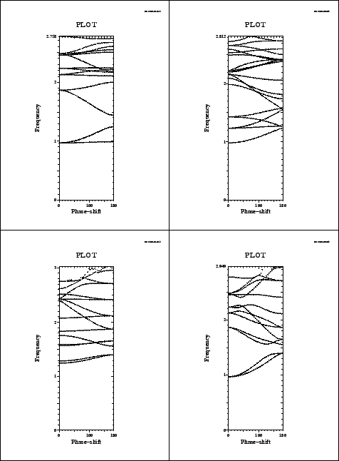
The resulting plots are presented in figure 5.9.

**Figure 5.9:** The four parts of the Brillouin diagram
$\begin{figure}\centerline{ \psfig{figure=brillo.part1-4.PS,width=10.5cm} }\end{figure}$

The following is the source of the program that combines the four parts of the Brillouin diagram to a single plot:

*
* /usr/local/gd1/examples-from-the-manual/a3dbrillo.f
*
* usage:
*
* cat brillo.part=[1-4].mtv | a.out
* mymtv2 3D-brillo.mtv
*
*
      DIMENSION f0(300,1 000), ph0(1 000)
      REAL, DIMENSION(100) :: Phase0, scale
      CHARACTER(LEN=1000) :: str
*
      i11= 11
      i19= 19
      OPEN (UNIT= i19
     1    , FILE= '3D-brillo.mtv')
*
      WRITE (UNIT= i19, FMT= 9000)
 9000 FORMAT(
     1 '$ DATA= CURVE2D NAME= "Brillouin-Diagramm"',/,
     2 '% linetype= 0',/,
     3 '% markertype= 3',/
     4 '% equalscale= false',/,
     5 '% fitpage= false',/,
     6 '% xyratio= 3',/,
     7 '% xlabel= "normalised Phase-shift"',/,
     8 '% ylabel= "Frequency"',/,
     9 '% comment= "no comment"',/
     x )
*
      af= 0.
      ap= 0.
*
      NMode= 10
*
      phase0(1:4)= (/ 0.0,
     1                1.0,
     2                2.0,
     3                4.0  /)
      scale(1:4)= (/ 1./180.0,    !! Gamma to H
     2               1./180.0,    !!     H to N
     3               1./180.0,    !!     N to P
     4              -1./180.0 /)  !!     P to Gamma
*
      Phase Last= 0.
      np= 1
      str= ' '
      DO
         DO
            IF (INDEX(str, '# phase:') .NE. 0) THEN
               jj= INDEX(str, '# phase:')+LEN('# phase:')
               READ (UNIT= str(jj:), FMT= *) phase
               IF (phase .LT. Phase Last) THEN
                  np= np+1
               ENDIF
               Phase Last= phase
               EXIT
            ENDIF
            READ (UNIT= *, FMT= '(A)', END= 10) str
         ENDDO
      write (*,*) ' phase:', phase
         pp= Phase0(np)
         ph0(np)= pp+phase*scale(np)
*
         mode= 0
         DO mode= 1, NMode, 1
            READ (UNIT= *, FMT= '(A)', END= 10) str
            READ (UNIT= str(2:), FMT= *, IOSTAT= iostat) f
            IF (iostat .NE. 0) EXIT
      write (*,*) ' pp, f:', pp+phase*scale(np), f
            f0(mode,np)= f
            WRITE  (UNIT= i19, FMT= 7010) pp+phase*scale(np),f
            af= MAX(af,f)
            ap= MAX(ap,pp+phase*scale(np))
         ENDDO
      ENDDO
   10 CONTINUE
*
 7010 FORMAT(
     1 '@ point x1=',E12.6,' y1=',E12.6,' z1= 0 markertype=1',
     2 ' markersize= 1')
*
      WRITE (UNIT= i19, FMT= *)
      WRITE (UNIT= i19, FMT= 9900) 0.,0.,0.,af,ap,af
 9900 FORMAT(3(' ',2(E12.6,' ')/),/)
*
      END

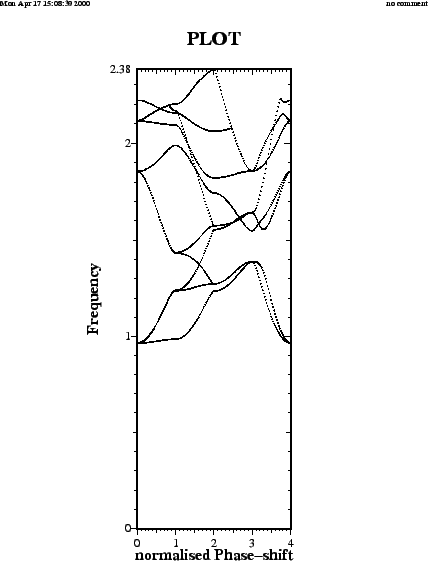
The resulting plot is presented in figure 5.10.

**Figure 5.10:** The four parts of the Brillouin diagram combined.
$\begin{figure}\centerline{ \psfig{figure=a3dbrillo.PS,width=10.5cm} }\end{figure}$

This is the end of this document

Up: Examples Previous: Scattering Parameters Contents